26. RNA-seq Analysis
26.1. Some basics
We are going to first talk about different needs in RNA-seq, from basics in library prep to the last steps of analyses.
How do you choose your library pipeline?
| Choice 1 | Choice 2 |
|---|---|
| More Replicates | Deeper Sequencing |
| RIN values < 7 | RNA values > 7 |
| ERCC | No ERCC |
| Poly A | Ribo depletion |
| Fragment size 1 | Fragment size 2 |
| Stranded | Non-stranded |
| Single end | Paired end |
| Short Read (50) | Medium Read (150) |
| Depth 1 | Depth 2 |
| RNA-seq | Targeted RNA-seq |
Biological vs Technical replicates
Schurch et al., 2016 “How many biological replicates are needed in an RNA-seq experiment and which differential expression tool should you use?”
How do you choose your bioinformatics pipeline?
| Choice 1 | Choice 2 |
|---|---|
| trimmomatic | cutadapt |
| Salmon, kallisto... | STAR, HISAT2, bowtie2 |
| DESeq2 | edgeR |
| clustering 1 (corr) | clustering 2 (PCA) |
| Pathway analysis | GSET |
| Visualization 1 | Visualization 100! |
| Upload them before paper submission! | Upload them before paper submission! |
26.2. Installations
We have installed the ‘heaviest’ packages that you need in this lesson in our Jetstream image. For future work, these are the installations that you will need, so that you have all of them together:
source("https://bioconductor.org/biocLite.R") # calls the package from the source
biocLite('Biobase') # newer versions of R use 'library()' as function instead of biocLite
install.packages("tidyverse") # we have this in our Image
library(tidyverse)
library(tximport)
library(DESeq2)
install.packages("devtools")
library(devtools)
install.packages('pheatmap')
library(RColorBrewer)
library(pheatmap)
biocLite("GOstats")
biocLite("org.Sc.sgd.db")
library(GOstats)
library(org.Sc.sgd.db)
26.3. Bioconductor
Bioconductor is a project to develop innovative software tools for use in computational biology. Bioconductor is an ‘umbrella package’ that includes many packages employed in biological analyses. Biobase is part of the Bioconductor project, and is used by many other packages. Biobase contains standardized data structures to represent genomic data. You can find help for Biobase typing:
browseVignettes("Biobase")
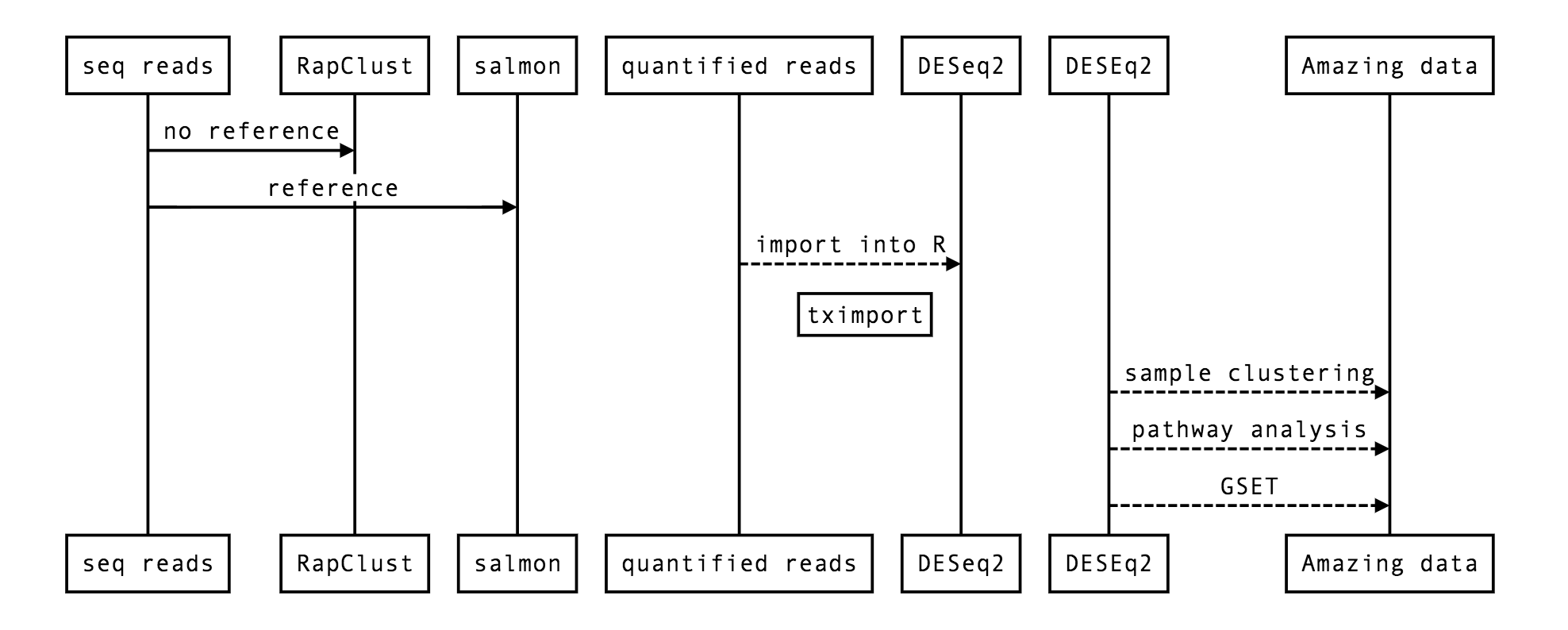
26.4. A simple RNA-seq flow
26.5. DESeq2
We are going to follow the lesson by Mike Love at DESeq2
This code chunk assumes that you have a count matrix called cts and a table of sample information called coldata. design indicates how to model the samples, here, we want to measure the effect of the condition, controlling for batch differences. The two factor variables batch and condition should then be columns of coldata.
dds <- DESeqDataSetFromMatrix(countData = cts,
                              colData = coldata,
                              design= ~ batch + condition)
dds <- DESeq(dds) # creates a DESeqDataSet
resultsNames(dds) # lists the coefficients
res <- results(dds, name="condition_trt_vs_untrt")
# or to shrink log fold changes association with condition:
res <- lfcShrink(dds, coef="condition_trt_vs_untrt", type="apeglm")
26.5.1. DESeqDataSet
DESeqDataSet class extends the RangedSummarizedExperiment class of the SummarizedExperiment package. Ranged referes here to counts associated with genomic ranges (exons) - we can then make use of other Bioconductor packages that explore range-based functionality (e.g. ChIP-seq peaks).
A DESeqDataSet must have a design formula: the variables that we will fit in the model to create our differential expression. The formula should be a tilde (~) followed by the variables with plus (+) signs between them (it will be coerced into an formula if it is not already).
Note: To get the most out of the package with default settings, put the variable of interest at the end of the formula and make sure the control level is the first level. The starting functions are:
If you have transcript quantification files, as produced by
Salmon,Sailfish, orkallisto, you would useDESeqDataSetFromTximport.If you have htseq-count files, the first line would use
DESeqDataSetFromHTSeq.If you have a
RangedSummarizedExperiment, the first line would useDESeqDataSet.
DESeq2 internally corrects for library size, so transformed or normalized values such as counts scaled by library size should not be used as input.
Depending on the upstream pipeline, a DESeqDataSet can be constructed using:
From transcript abundance files and
tximport- this is the pipeline that we will use in this tutorialFrom a
count matrixFrom
htseq-countfilesFrom a
SummarizedExperimentobject
26.5.2. Transcript abundance files: tximport
You can import transcript abundance files from salmon, sailfish, kallisto and RSEM using tximport, which will create gene-level count matrices for use with DESeq2.
Advantages:
correction for potential changes in gene length across samples (e.g. from differential isoform usage) (Trapnell et al. 2013);
Salmon,Sailfishandkallistoare substantially faster and require less memory and disk usage compared to alignment-based methods that require creation and storage of BAM files;it is possible to avoid discarding fragments that can align to multiple genes with homologous sequence, thus increasing sensitivity (Robert and Watson 2015).
Note: the tximport-to-DESeq2 approach uses estimated gene counts from the transcript abundance quantifiers, but not normalized counts.
26.5.3. Organise your directory to work on it!
Log into your Jetstream Instance and lauch R Studio. We will use both the Console (for R) and the Terminal (for bash) there.
We are first going to make a new directory using the Terminal where we will be doing all the analysis, called rna_seq_r, where we will create tow other directories called figures and r_script:
mkdir rna_seq_r
cd rna_seq_r
mkdir figures
mkdir r_script
We are going to set our working directory in the R Console so that we can find and store all our analysis there:
setwd(~/rna_seq_r)
This is how you start any project in R: set your working directory, where you will find your input files (unless you download them directly as in this lesson) and where you will output all your data (and your RScript!).
26.6. Continue the lesson in RMarkdown
We are now going to download the rest of the lesson and follow it on RMarkdown, which is a great way of making and sharing documents. Type in your Terminal:
wget https://raw.githubusercontent.com/maggimars/YeastTutorial/master/R_RNA.Rmd
and let’s get started!