24. Annotating and evaluating a de novo transcriptome assembly
At the end of this lesson, you will be familiar with:
how to annotate a de novo transcriptome assembly
parse GFF3 output from the annotation output to use for DE analysis
several methods for evaluating the completeness of a de novo transcriptome assembly
What a Jupyter notebook is and how to execute a few commands in Python
24.1. Annotation with dammit
dammit!
dammit is an annotation pipeline written by Camille Scott. The dammit pipeline runs a relatively standard annotation protocol for transcriptomes: it begins by building gene models with Transdecoder, then uses the following protein databases as evidence for annotation:
Pfam-A, Rfam, OrthoDB, uniref90 (uniref is optional with--full).
If a protein dataset for your organism (or a closely-related species) is available, this can also be supplied to the dammit pipeline with the --user-databases as optional evidence for the annotation.
In addition, BUSCO v3 is run, which will compare the gene content in your transcriptome with a lineage-specific data set. The output is a proportion of your transcriptome that matches with the data set, which can be used as an estimate of the completeness of your transcriptome based on evolutionary expectation (Simho et al. 2015).
There are several lineage-specific datasets available from the authors of BUSCO. We will use the metazoa dataset for this transcriptome.
24.1.1. Installation
Annotation necessarily requires a lot of software! dammit attempts to simplify this and make it as reliable as possible, but we still have some dependencies.
dammit can be installed via bioconda, but the latest version is not up there yet. Let’s download a working conda environment.yml file that will help us install the latest version of dammit.
cd
curl -L https://raw.githubusercontent.com/dib-lab/elvers/master/elvers/rules/dammit/environment.yml -o dammit-env.yaml
Now let’s build an environment from that yaml file:
conda env create -f dammit-env.yml -n dammit-env
conda activate dammit-env
To make sure your installation was successful, run
dammit -h
This will give a list of dammit’s commands and options:
The version (dammit --version) should be:
dammit 1.1
24.1.1.1. Database Preparation
dammit has two major subcommands: dammit databases and dammit annotate. The databases command checks that databases are installed and prepared, and if run with the --install flag,
it will perform that installation and preparation. If you just run dammit databases on its own, you should get a notification that some database tasks are not up-to-date. So, we need
to install them!
Install databases (this will take a long time, usually >10 min):
dammit databases --install --busco-group metazoa
Note: dammit installs databases in your home directory by default. If you have limited space in your home directory or on your instance, you can install these databases in a different location (e.g. on an external volume) by running dammit databases --database-dir /path/to/install/databases before running the installation command.
We used the “metazoa” BUSCO group. We can use any of the BUSCO databases, so long as we install them with the dammit databases subcommand. You can see the whole list by running
dammit databases -h. You should try to match your species as closely as possible for the best results. If we want to install another, for example:
dammit databases --install --busco-group protists
Phew, now we have everything installed!
Now, let’s take a minute and thank Camille for making this process easy for us by maintaining a recipe on bioconda. This saves us a lot of hassle with having to install individual parts required for the pipeline. AND on top of the easy installation, there is this slick pipeline! Historically, transcriptome annotation involved many tedious steps, requiring bioinformaticians to keep track of parsing databases alignment ouptut and summarizing across multiple databases. All of these steps have been standardized in the dammit pipeline, which uses the pydoit automation tool. Now, we can input our assembly fasta file -> query databases -> and get output annotations with gene names for each contig - all in one step. Thank you, Camille!
24.1.2. Annotation
Keep things organized! Let’s make a project directory:
cd ~/
mkdir -p ~/annotation
cd ~/annotation
Let’s copy in the trinity assembly file we made earlier:
cp ../assembly/nema-trinity.fa ./
Now we’ll download a custom Nematostella vectensis protein database. Somebody has already created a proper database for us Putnam et al. 2007 (reference proteome available through uniprot). If your critter is a non-model organism, you will likely need to grab proteins from a closely-related species. This will rely on your knowledge of your system!
curl -LO ftp://ftp.uniprot.org/pub/databases/uniprot/current_release/knowledgebase/reference_proteomes/Eukaryota/UP000001593_45351.fasta.gz
gunzip -c UP000001593_45351.fasta.gz > nema.reference.prot.faa
rm UP000001593_45351.fasta.gz
Run the command:
dammit annotate nema-trinity.fa --busco-group metazoa --user-databases nema.reference.prot.faa --n_threads 6
While dammit runs, it will print out which task it is running to the terminal. dammit is written with a library called pydoit, which is a python workflow library similar to GNU Make. This not only helps organize the underlying workflow, but also means that if we interrupt it, it will properly resume!
After a successful run, you’ll have a new directory called trinity.nema.fasta.dammit. If you
look inside, you’ll see a lot of files:
ls nema-trinity.fa.dammit/
Expected output:
annotate.doit.db                    nema-trinity.fa.transdecoder.cds                    nema-trinity.fa.x.nema.reference.prot.faa.crbl.gff3            nema-trinity.fa.x.sprot.best.csv
dammit.log                          nema-trinity.fa.transdecoder.gff3                   nema-trinity.fa.x.nema.reference.prot.faa.crbl.model.csv       nema-trinity.fa.x.sprot.best.gff3
nema-trinity.fa                     nema-trinity.fa.transdecoder.pep                    nema-trinity.fa.x.nema.reference.prot.faa.crbl.model.plot.pdf  nema-trinity.fa.x.sprot.maf
nema-trinity.fa.dammit.fasta        nema-trinity.fa.transdecoder_dir                    nema-trinity.fa.x.pfam-A.csv                                   run_nema-trinity.fa.metazoa.busco.results
nema-trinity.fa.dammit.gff3         nema-trinity.fa.x.OrthoDB.best.csv                  nema-trinity.fa.x.pfam-A.gff3                                  tmp
nema-trinity.fa.dammit.namemap.csv  nema-trinity.fa.x.OrthoDB.best.gff3                 nema-trinity.fa.x.rfam.gff3
nema-trinity.fa.dammit.stats.json   nema-trinity.fa.x.OrthoDB.maf                       nema-trinity.fa.x.rfam.tbl
nema-trinity.fa.transdecoder.bed    nema-trinity.fa.x.nema.reference.prot.faa.crbl.csv  nema-trinity.fa.x.rfam.tbl.cmscan.out
The most important files for you are nema-trinity.fa.dammit.fasta,
nema-trinity.fa.dammit.gff3, and nema-trinity.fa.dammit.stats.json.
If the above dammit command is run again, there will be a message:
**Pipeline is already completed!**
24.1.3. Parse dammit output
Camille wrote dammit in Python, which includes a library to parse gff3 dammit output. To send this output to a useful table, we will need to open the Python environment.
To do this, we will use a Jupyter notebook. In addition to executing Python commands, Jupyter notebooks can also run R (as well as many other languages). Similar to R markdown (Rmd) files, Jupyter notebooks can keep track of code and output. The output file format for Jupyter notebooks is .ipynb, which GitHub can render. See this gallery of interesting Jupyter notebooks.
Let’s open python in our terminal!
python
This opens python in your terminal, allowing you to run commands in the python language.
Let’s import the libraries we need.
import pandas as pd
from dammit.fileio.gff3 import GFF3Parser
Now enter these commands:
gff_file = "nema-trinity.fa.dammit/nema-trinity.fa.dammit.gff3"
annotations = GFF3Parser(filename=gff_file).read()
names = annotations.sort_values(by=['seqid', 'score'], ascending=True).query('score < 1e-05').drop_duplicates(subset='seqid')[['seqid', 'Name']]
new_file = names.dropna(axis=0,how='all')
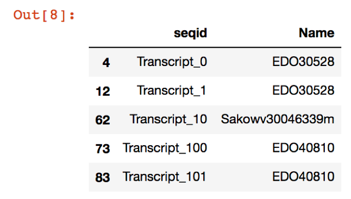
new_file.head()
Which will give an output that looks like this:
Try commands like,
annotations.columns
and
annotations.head()
or
annotations.head(50)
**Questions
What do these commands help you to see?
How might you use this information to modify the
namesline in the code above?
To save the file, add a new cell and enter:
new_file.to_csv("nema_gene_name_id.csv")
Now, we can return to the bash terminal, type:
quit()
We can look at the output we just made, which is a table of genes with ‘seqid’ and ‘Name’ in a .csv file: nema_gene_name_id.csv.
less nema_gene_name_id.csv
Notice there are multiple transcripts per gene model prediction. This .csv file can be used in tximport as a tx2gene file in downstream DE analysis.
24.2. Evaluation with BUSCO
BUSCO aims to provide a quantitative measure of transcriptome (or genome/gene set) completeness by searching for near-universal single-copy orthologs. These ortholog lists are curated into different groups (e.g. genes found universally across all metazoa, or all fungi, etc), and are currently based off of OrthoDB v9.
Metazoa database used with 978 genes
“Complete” lengths are within two standard deviations of the BUSCO group mean length
Useful links:
Website: http://busco.ezlab.org/
Paper: Simao et al. 2015
24.2.1. Run the command:
We’ve already installed and ran the BUSCO command with the dammit pipeline. Let’s take a look at the results.
Check the output:
cat nema-trinity.fa.dammit/run_nema-trinity.fa.metazoa.busco.results/short_summary_nema-trinity.fa.metazoa.busco.results.txt
Challenge: How do the BUSCO results of the full transcriptome compare?
Run the BUSCO command by itself:
run_BUSCO.py \
-i nema-trinity.fa \
-o nema_busco_metazoa -l ~/.dammit/databases/busco2db/metazoa_odb9 \
-m transcriptome --cpu 4
When you’re finished, exit out of the conda environment:
conda deactivate