11. R and RStudio introduction
11.1. Using RStudio on Jetstream
We will be using R and RStudio on our cloud instances. We have pre-installed RStudio on the workshop image. Start up a Jetstream m1.medium or larger using the ANGUS 2019 image as per Jetstream startup instructions. Connect to your instance.
We will need our instance username to connect to RStudio. To determine what your username is, run:
echo My username is $USER
The link for the RStudio server interface is built with our instance’s IP address (by default in port 8787), which we can get from the terminal by running the following command:
echo http://$(hostname -i):8787/
hostnameis a command in the terminal that will get various information about our computers. Using it with the-ioption returns our computer’s IP address. So surrounding it within parentheses preceded by the$means the command line will execute that command first, put the output of that command in it’s place (our IP address), and then run theechocommand which then prints out the proper link to our RStudio server 😊
Now go to the web address printed to your terminal in your Web browser, which should look something like this:
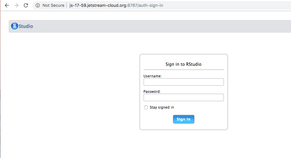
and log in with the username and password we will provide.
11.2. Installing on your own computer:
We will be using R and RStudio in the cloud. To use RStudio on your computer, you can download R and RStudio. If you do not have R and RStudio installed:
Download R from CRAN:https://cran.r-project.org/
Go to RStudio download page and install the version that is compatible with your operating system: https://www.rstudio.com/products/rstudio/download/#download This link provides futher instructions on installing and setting up R and RStudio on your computer.
11.3. Introduction to R and RStudio
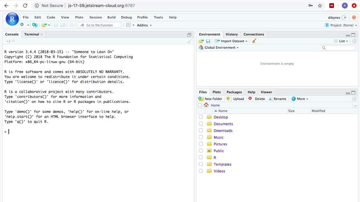
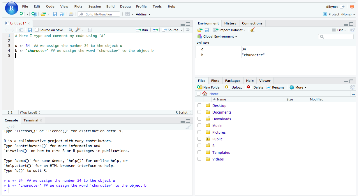
R is a programming language and free software environment for statistical computing and graphics. Many bioinformatics programs are implemented in R. RStudio is a graphical integrated development environment (IDE) that displays and organizes more information about R. R is the underlying programming language. Once you start RStudio, you see this layout (it will be similar either on your instance or on your computer):
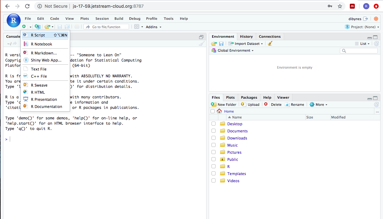
Scripts are like a digital lab book. They record everything your run, as
well as notes to yourself about how and why you ran it. To start a new
script you can click on the icon that looks like a page with a ‘+’
underneath File and select –>R script. This generates a .R file.
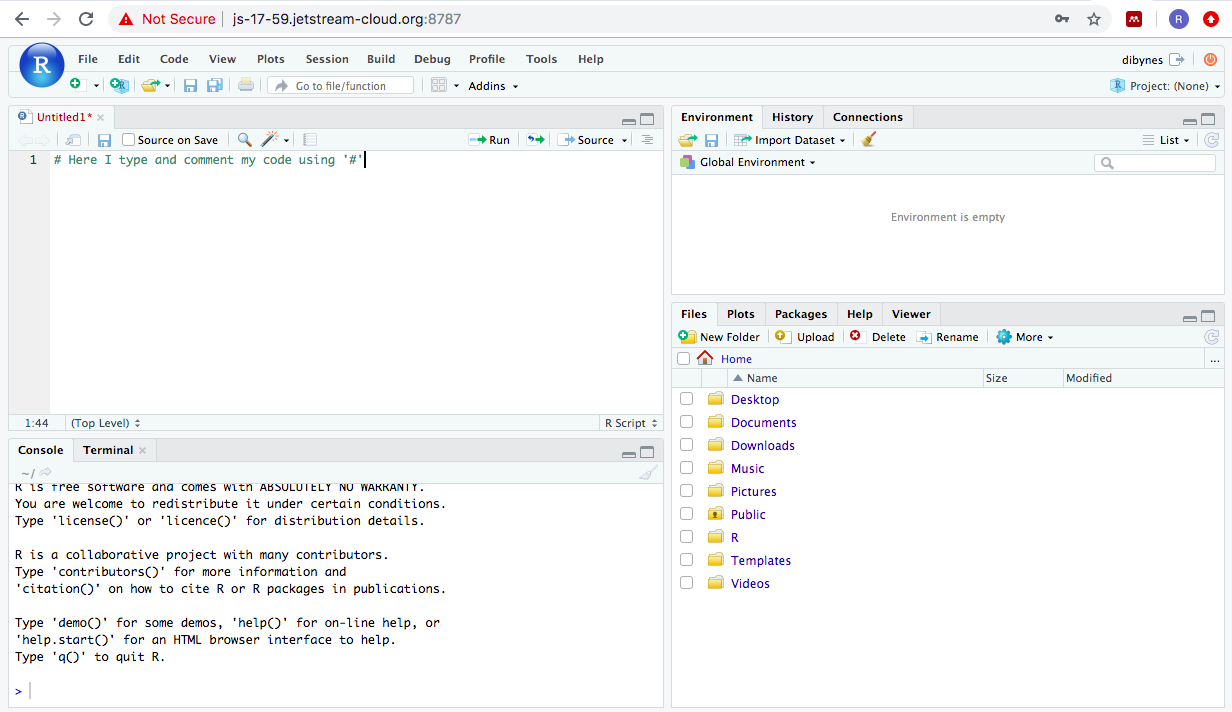
.R files are plain text files that use the file extension .R so that
humans can remember that the file contains R code.
Although scripts are a record of our code, they also include comments about our code. These comments are very important as they remind your future self (and whoever you pass your script) why you did what you did. Think of comments like the notes you take in your lab book when you do experiments.
When you execute a line of your script, it is sent to the console. While the script is a permanent record of everything you ran, the console is the engine that runs those things. You can run code from a script or the console, but it is only recorded in scripts.
There are two additional panes in RStudio:
Environment/History/Connections pane
Environment Pane: This pane records the objects that are currently loaded in our RStudio environment. This includes any data object that we created and the basic information about them.
History Pane: This has output similar to the
historycommand that we used in the shell. It records all of the commands that we have executed in the R console.
Files/Plots/Packages/Help/Viewer pane provides a space for us to interact with plots and files we create and with built-in help files in R.
Packages Pane: A place to organize the packages within RStudio. Allows easy installation or loading (
library()) of the packages we have.
And now we’re ready to start the fun part!
11.4. Basic concepts
11.4.1. Objects
An R object is something that you create and assign a value or function
to. You do this using the assignment operator which is <- (NOTE:
shortcut Alt + -). For example you can assign a numeric value to an
object by typing in your script (remember to comment what you are
doing):
a <- 34 # assign the number 34 to the object a
You can also assign a character value to an object:
b <- 'mouse' # assign the word 'character' to the object b
To run a line of code, put your cursor on the line that you want to run
and press Enter+Cmd or Enter+Ctrl. Or select the line and click the
button that says Run on the right top corner of your script.
Now check your Console and Environment tabs, you will see that the commands have run and that you have created new objects!
You can do all sorts of stuff with your objects: operations,
combinations, use them in functions. Below we show how to perform
multiplication using an object. Because a stores the value 34, we
can multiply it by 2:
a2 <- a*2 # multiply a by 2
11.4.2. Functions and Arguments
Functions are “canned scripts” that automate more complicated sets of
commands including operations assignments, etc. Many functions are
predefined, or can be made available by importing R packages (more on
that later). A function usually takes one or more inputs called
arguments. Functions often (but not always) return a value. A typical
example would be the function sqrt(). The input (the argument) must be
a number, and the return value (in fact, the output) is the square root
of that number. Executing a function (‘running it’) is called calling
the function. An example of a function call is:
sqrt(a) ## calculate the square root of a
Here, the value of a is given to the sqrt() function, the sqrt()
function calculates the square root, and returns the value which is then
assigned to the object b. This function is very simple, because it
takes just one argument.
The return ‘value’ of a function need not be numerical (like that of
sqrt()), and it also does not need to be a single item: it can be a
set of things, or even a dataset. We’ll see that when we read data files
into R.
Similar to the shell, arguments can be anything, not only numbers or filenames, but also other objects. Exactly what each argument means differs per function, and must be looked up in the documentation (see below). Some functions take arguments which may either be specified by the user, or, if left out, take on a default value: these are called options. Options are typically used to alter the way the function operates, such as whether it ignores ‘bad values’, or what symbol to use in a plot. However, if you want something specific, you can specify a value of your choice which will be used instead of the default.
Let’s try a function that can take multiple arguments: round().
round(3.141592) ## round number
Arguments are the ‘conditions’ of a function. For example, the function
round() has an argument to determine the number of decimals, and its
default in R is 0. Here, we’ve called round() with just one argument,
3.14159, and it has returned the value 3. That’s because the default is
to round to the nearest whole number. If we want more digits we can see
how to do that by getting information about the round function. We can
use args(round) to find what arguments it takes, or look at the help for
this function using ?round.
args(round) ## show the arguments of the function 'round'
?round ## shows the information about 'round'
We can change this to two decimals by changing the digits argument:
round(3.141592, digits = 2)
Note that we do not need to specify the name of the argument as R detects this by the position within the function:
round(3.141592, 2)
Though, it is preferablt to show the argument names. Plus, we have the added benefit of having the ability to change the order of the arguments if the arguments are named:
round(digits = 2, x= 3.141592)
It’s best practice to put the non-optional arguments (the data that you want the function to work on) first, and then specify the names of all optional arguments. This helps other to interpret your code more easily.
11.4.3. Vectors
A vector is the most common and basic data type in R, and is pretty much the workhorse of R. A vector is composed by a series of values, which can be either numbers or characters. We can assign a series of values to a vector using the c() function.
yeast_strain <- c('WT','snf2')
concentration <- c(43.903, 47.871)
There are many functions to inspect a vector and get information about its contents:
length(yeast_strain) # number of elements in a vector
class(concentration) # type of object b
str(yeast_strain) # inspect the structure of a
11.4.4. Data types
An atomic vector is the simplest R data type, and it is a vector of a single type. The 6 main atomic vector types that R uses are:
'character'letters or words'numeric'(ordouble) for numbers'logical'forTRUEandFALSE(booleans)'integer'for integer numbers (e.g.,2L, theLindicates to R that it’s an integer)'complex'to represent complex numbers with real and imaginary parts, for example2 + 4i'raw'for bitstreams that we will not use or discuss furtherfactorrepresents categorical data (more below!)
You can check the type of vecor you are using with the typeof()
function.
typeof(concentration)
Challenge: Atomic vectors can be a character, numeric (or double), integer, and logical. But what happens if we try to mix these types in a single vector?
Solution
yeast_strain_concentration <- c(yeast_strain, concentration) # combine two vectors
yeast_strain_concentration
## [1] "WT" "snf2" "43.903" "47.871"
# Solution: All indices are "coerced" to the same "type", e.g. character.
logical → numeric → character ← logical
R uses many data structures, the main ones are:
vectorcontain elements of the same type in one dimensionlistcan contain elements of different types and multiple data structuresdata.framecontains rows and columns. Columns can contain different types from other columns.matrixwith rows and columns that are of the same typearraystores data in more than 2 dimensions
We will use vectors, matrices, data.frames, and factors today.
11.4.5. Subsetting
We can extract values from a vector based on position or conditions:
this is called subsetting. One way to subset in R is to use [].
Indices start at 1.
strains <-  c('WT', 'snf2', 'snf1', 'snf1_snf2')
strains[2] # subsets the second element
strains[c(2,3)] # subsets the second and third elements
more_strains <- strains[c(1, 2, 3, 1, 4, 3)] # to create an object with more elements than tha original one
more_strains
11.4.5.1. Conditional subsetting
We can also subset based on conditions, using a logical vector with
TRUE and FALSE or with operators:
strains[c(TRUE, FALSE, FALSE, TRUE)]
concentration >= 43
concentration > 40
concentration < 47
concentration <= 47
concentration[ concentration < 45 | concentration > 47] # | is OR
concentration[ concentration < 45 & concentration == 47] # & is AND , == is mathematical 'equal'
more_strains[more_strains %in% strains]
11.4.6. Missing data
As R was designed to analyze datasets, it includes the concept of missing data (which is uncommon in other programming languages). Missing data are represented in vectors as NA.
There are in-built functions and arguments to deal with missing data. For example, this vector contains missing data:
concentration <- c(43.903, 47.871, NA, 48.456, 53.435)
We can use the following functions to remove or ignore it:
mean(concentration, na.rm = TRUE) # mean of concentration removing your NA
concentration[!is.na(concentration)] # extract all elements that are NOT NA
na.omit(concentration) # returns a 'numeric' atomic vector with incomplete cases removed
concentration[complete.cases(concentration)] # returns a 'numeric' atomic vector with elements that are complete cases
Note, if your data includes missing values, you can code them as blanks (”“), or as”NA” before reading them into R.
11.4.7. Factors
Factors represent categorical data. They are stored as integers associated with labels and they can be ordered or unordered. While factors look (and often behave) like character vectors, they are actually treated as integer vectors by R. So you need to be very careful when treating them as strings.
strains <-  factor(c('WT', 'snf2', 'snf1', 'snf1_snf2')) # We make our strains object a factor
class(strains)
nlevels(strains)
strains # R orders alphabetically
Once created, factors can only contain a pre-defined set of values,
known as levels. By default, R always sorts levels in alphabetical
order. We can reorder them using the levels argument.
strains <- factor(strains, levels = c('WT', 'snf1', 'snf2', 'snf1_snf2')) # we reorder them as we want them
strains
We convert objects using as.XXX functions:
strains <- as.character(strains)
class(strains)
strains <- as.factor(strains)
class(strains)
And we can also rename factors based on position:
levels(strains)[4] <- 'wild_type'
11.5. Starting with tabular data
This tutorial is a continuation from our Salmon lesson – we are using sequencing data European Nucleotide Archive dataset PRJEB5348. This is an RNA-seq experiment using comparing two yeast strains, SFF2 and WT. Although we’re only working with 6 samples, this was a much larger study. They sequenced 96 samples in 7 different lanes, with 45 wt and 45 mut strains. Thus, there are 45 biological replicates and 7 technical replicates present, with a total of 672 samples! The datasets were compared to test the underlying statistical distribution of read counts in RNA-seq data, and to test which differential expression programs work best.
We will get the information about the RNA quality and quantity that the authors measured for all of their samples, and we will explore how the authors made their data avaialble and ‘linkable’ between technical and biological replicates.
We are going to explore those datasets using RStudio, combining a both base R and an umbrella package called tidyverse.
library('tidyverse')
First we are going to read the files from a url and assign that to
experiment_info, using read_tsv():
experiment_info <- read_tsv(file = 'https://osf.io/pzs7g/download/')
Let’s investigate your new data using some exploratory functions:
class(experiment_info) # type of object that sample_details is
dim(experiment_info) # dimensions
summary(experiment_info) # summary stats
head(experiment_info) # shows the first 6 rows and all columns
tail(experiment_info) # last 6 rows and all columns
str(experiment_info) # structure
What do you notice? The last 4 columns are empty! We can get rid of them by subsetting, and having a look that we have done things correctly:
sum(is.na(experiment_info$X10)) # checks how many NAs the column X10 has so that you know all your rows are NAs (or not!)
experiment_info <- experiment_info[ , 1:9] # subset all rows and columns 1 to 9
Challenge: How many columns are in the experiment_info data frame
now?
Solution
dim(experiment_info) # dimensions
experiment_info <- rename(experiment_info, units = X9)
11.5.1. Manipulating data with dplyr
We can now explore this table and reshape it using dplyr. We will
cover in this lesson:
%>%: pipes, they allow ‘concatenating’ functionsselect(): subsets columnsfilter(): subsets rows on conditionsmutate(): create new columns using information from other columnsgroup_by()andsummarize(): create summary statistics on grouped dataarrange(): sort resultscount(): counts discrete values
11.5.2. Selecting columns and filtering rows
We have now a table with many columns – but what if we don’t need all of
the columns? We can select columns using select, which requires the
names of the colums that you want to keep as arguments:
# Let's confirm the arguments by looking at the help page
?select # Notice how the help page is different from the shell manual pages?

# Now lets select specific columns
select(experiment_info, Sample, Yeast Strain, Nucleic Acid Conc., Sample, 260/280, Total RNA)
What happened? R cannot parse the spaces in the column names properly.
We can add back commas around the name of the column. These tell R
that these words belong together:
select(experiment_info, Sample, `Yeast Strain`, `Nucleic Acid Conc.`, 260/280, `Total RNA`)
Also, R gets confused when column names start with a number. So, we will also need to specify where the numbers start and stop:
select(experiment_info, Sample, `Yeast Strain`, `Nucleic Acid Conc.`, `260/280`, `Total RNA`)
So let’s store that in an object named experiment_info:
experiment_info <- select(experiment_info, Sample, `Yeast Strain`, `Nucleic Acid Conc.`, A260, A280, `260/280`, `Total RNA`)
NOTE: When choosing names from columns, make sure that you are consistent and choose something simple, all lowercase, all uppercase, or CamelCase. Having spaces in column makes it hard for R to deal with, and can lead to unexpected results or silent errors.
We select all columns except for by using - before the name of the
columns we do not want to include, for example all columns except for
A260 and A280:
# Remove two columns: A260 and A280
select(experiment_info, -A260, -A280)
The filter function works on rows, so we can also filter the data
based on conditions in a column:
filter(experiment_info, `Nucleic Acid Conc.` > 1500)
11.5.3. Exercise 1
Select the columns
Sample,Yeast Strain,A260andA280and assign that to a new object calledexperiment_data.
Solution #1
experiment_data <-  select(experiment_info, Sample, `Yeast Strain`, A260, A280)
head(experiment_data)
## # A tibble: 6 x 4
##   Sample `Yeast Strain`  A260  A280
##    <dbl> <chr>          <dbl> <dbl>
## 1      1 snf2            43.9  19.9
## 2      2 snf2            47.9  22.1
## 3      3 snf2            34.5  15.6
## 4      4 snf2            34.0  15.4
## 5      5 snf2            28.1  12.7
## 6      6 snf2            48.2  22.1
11.5.4. Exercise 2
Filter rows for only WT strains that had more than 1500 ng/uL concentration and make a new tibble called wild_type.
Solution #2
wild_type <- filter(experiment_info, `Yeast Strain` %in% 'WT' & `Nucleic Acid Conc.` > 1500)
head(wild_type)
## # A tibble: 6 x 7
##   Sample `Yeast Strain` `Nucleic Acid Co…  A260  A280 `260/280` `Total RNA`
##    <dbl> <chr>                      <dbl> <dbl> <dbl>     <dbl>       <dbl>
## 1     49 WT                         2052.  51.3  23.6      2.17        61.6
## 2     50 WT                         1884.  47.1  21.6      2.18        56.5
## 3     51 WT                         2692.  67.3  30.6      2.2         80.8
## 4     52 WT                         3022   75.5  34.3      2.2         90.7
## 5     53 WT                         3235   80.9  36.9      2.19        97.0
## 6     54 WT                         3735.  93.4  43.2      2.16       112.
11.5.5. Pipes
What if we want to select and filter at the same time? We use a
“pipe” in R, which is represented by %>%. Note: This is the R
version of the shell “redirector” |!
Pipes are available via the magrittr package, installed automatically
with dplyr. If you use RStudio, you can type the pipe with
Ctrl + Shift + M if you have a PC or Cmd + Shift + M if you have a
Mac as a shortcut to get to produce a pipe.
We can combine the two subsetting activities from Exercise 1 and 2 using
pipes %>% :
experiment_info_wt <- experiment_info %>%
  filter(`Yeast Strain` == 'WT' & `Nucleic Acid Conc.` > 1500) %>%
  select(Sample, `Yeast Strain`, A260, A280)
11.5.6. Exercise 3
Using pipes, subset experiment_info to include all the samples that had a concentration less than 1500 and where total RNA was more or equal than 40 ug and retain only the columns that tell you the sample, yeast strain, nucleic acid concentration and total RNA. Assign that to a new table called samples_sequenced.
Solution #3
samples_sequenced <- experiment_info %>%
  filter(`Nucleic Acid Conc.` < 1500 & `Total RNA` >= 40) %>%
  select(Sample, `Yeast Strain`,`Nucleic Acid Conc.`,`Total RNA`)

samples_sequenced
## # A tibble: 5 x 4
##   Sample `Yeast Strain` `Nucleic Acid Conc.` `Total RNA`
##    <dbl> <chr>                         <dbl>       <dbl>
## 1      3 snf2                          1379.        41.4
## 2      4 snf2                          1359.        40.8
## 3     22 snf2                          1428.        42.8
## 4     24 snf2                          1386.        41.6
## 5     90 WT                            1422.        42.7
11.5.7. Mutate
What if I want to create a new column? I use the function mutate for
this. Let’s convert our units into micrograms/microliter:
experiment_info %>%
  mutate(concentration_ug_uL = `Nucleic Acid Conc.` / 1000)
Or create more than one column! And pipe that into head so that we have a peep:
experiment_info %>%
  mutate(concentration_ug_uL = `Nucleic Acid Conc.` / 1000,
          half_concentration = concentration_ug_uL / 1000) %>%
  head()
11.5.8. Exercise 4
Create a new table called library_start that includes the columns sample, yeast strain and two new columns called RNA_100 with the calculation of microliters to have 100ng of RNA and another column called water that says how many microliters of water we need to add to that to reach 50uL.
Solution #4
library_start <- experiment_info %>%
  mutate(RNA_100 = 100/ `Nucleic Acid Conc.`,
          water = 50 - RNA_100) %>%
  select(Sample, `Yeast Strain`, RNA_100, water)

head(library_start)
## # A tibble: 6 x 4
##   Sample `Yeast Strain` RNA_100 water
##    <dbl> <chr>            <dbl> <dbl>
## 1      1 snf2            0.0569  49.9
## 2      2 snf2            0.0522  49.9
## 3      3 snf2            0.0725  49.9
## 4      4 snf2            0.0736  49.9
## 5      5 snf2            0.0891  49.9
## 6      6 snf2            0.0519  49.9
11.5.9. Exercise 5
Pretty difficult to pipette! Can redo the table considering that you have done a 1:10 dilution of your samples? Include the columns of A260 and A280 values in addition to sample, yeast strain, RNA_100 and water.
Solution #5
library_start_diluted <-  experiment_info %>%
  mutate(diluted_RNA = 1000/ `Nucleic Acid Conc.`,
          water = 50 - diluted_RNA) %>%
  select(Sample, `Yeast Strain`, `A260`, `A280`, diluted_RNA, water)

head(library_start_diluted)
## # A tibble: 6 x 6
##   Sample `Yeast Strain`  A260  A280 diluted_RNA water
##    <dbl> <chr>          <dbl> <dbl>       <dbl> <dbl>
## 1      1 snf2            43.9  19.9     0.00569  50.0
## 2      2 snf2            47.9  22.1     0.00522  50.0
## 3      3 snf2            34.5  15.6     0.00725  50.0
## 4      4 snf2            34.0  15.4     0.00736  50.0
## 5      5 snf2            28.1  12.7     0.00891  50.0
## 6      6 snf2            48.2  22.1     0.00519  50.0
11.5.10. Exercise 6
Based on the tibble library_start_diluted, create a new tibble called
seq_samplesthat includes only samples with a A260/A280 ratio of 2.2 or more and that only contains the columns for sample, yeast strain, A260280 ratio, diluted RNA and water.
Solution #6
seq_samples <- library_start_diluted %>%
  mutate(A260_A280 = `A260`/`A280`) %>%
  filter(A260_A280 >= 2.2) %>%
  select(Sample, `Yeast Strain`, A260_A280, diluted_RNA, water)

head(seq_samples)
## # A tibble: 6 x 5
##   Sample `Yeast Strain` A260_A280 diluted_RNA water
##    <dbl> <chr>              <dbl>       <dbl> <dbl>
## 1      1 snf2                2.21     0.00569  50.0
## 2      3 snf2                2.21     0.00725  50.0
## 3      4 snf2                2.21     0.00736  50.0
## 4      5 snf2                2.22     0.00891  50.0
## 5      7 snf2                2.21     0.00991  50.0
## 6     11 snf2                2.20     0.00963  50.0
11.5.11. Split-apply-combine
The approach of split-apply-combine allows you to split the data into
groups, apply a function/analysis and then combine the results. We
can do this usign group_by() and summarize().
group_by() takes as argument the column names that contain
categorical variables that we want to calculate summary stats for. For
example, to determine the average RNA concetration per strain:
experiment_info %>%
  group_by(`Yeast Strain`) %>%
  summarize(mean_concentration = mean(`Nucleic Acid Conc.`))
or summarize using more than one column:
experiment_info %>%
  group_by(`Yeast Strain`) %>%
  summarize(mean_concentration = mean(`Nucleic Acid Conc.`),
            mean_total_RNA = mean(`Total RNA`))
NOTE: Our table does not have missing values. However, we have built-in functions in R that can deal with this. We can filter values that are not NA:
experiment_info %>%
  group_by(`Yeast Strain`) %>%
  summarize(mean_concentration = mean(`Nucleic Acid Conc.`, na.rm = TRUE), # remove NA values
            mean_total_RNA = mean(`Total RNA`))

experiment_info %>%
  filter(!is.na(`Nucleic Acid Conc.`)) %>%   # filter to keep only the values that are not NAs
  group_by(`Yeast Strain`) %>%
  summarize(mean_concentration = mean(`Nucleic Acid Conc.`),
            mean_total_RNA = mean(`Total RNA`))
We can now arrange the data in ascending order (default of arrange())
or descending using desc():
experiment_info %>%
  filter(!is.na(`Nucleic Acid Conc.`)) %>%  # filter to keep only the values that are not NAs
  group_by(`Yeast Strain`) %>%
  summarize(mean_concentration = mean(`Nucleic Acid Conc.`),
            mean_total_RNA = mean(`Total RNA`)) %>%
  arrange(mean_concentration) # arrange new table in ascending mean concentrations

experiment_info %>%
  filter(!is.na(`Nucleic Acid Conc.`)) %>%  # filter to keep only the values that are not NAs
  group_by(`Yeast Strain`) %>%
  summarize(mean_concentration = mean(`Nucleic Acid Conc.`),
            mean_total_RNA = mean(`Total RNA`)) %>%
  arrange(desc(mean_concentration)) # arrange new table in descending mean concentrations
Another useful function is count() to count categorical values:
experiment_info %>%
  count(`Yeast Strain`)
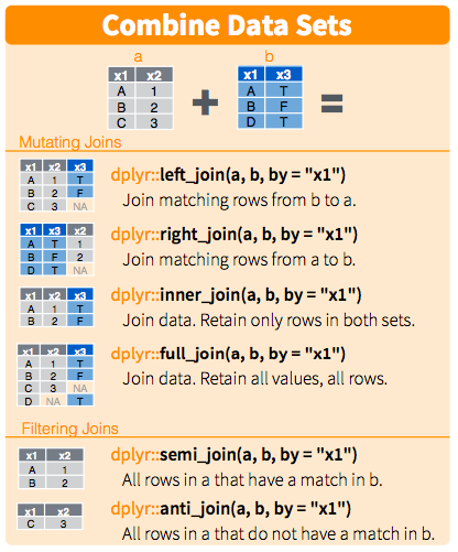
11.5.12. Combining Datasets using join
On many ocassions we will have more than one table that we need to
extract information from. We can easily do this in R using the family of
join functions.
We are going to first download extra information about the samples that we are are investigating and assigning them to an object called ena_info:
ena_info <- read_tsv(file = 'https://osf.io/6s4cv/download')
sample_mapping <- read_tsv(file = 'https://osf.io/uva3r/download')
11.5.13. Exercise 7
Explore your new dataset ena_info and sample_mapping. What commands can you use?
Solution #7
head(ena_info)
## # A tibble: 6 x 14
##   study_accession run_accession tax_id scientific_name instrument_model
##   <chr>           <chr>          <dbl> <chr>           <chr>
## 1 PRJEB5348       ERR458493       4932 Saccharomyces … Illumina HiSeq …
## 2 PRJEB5348       ERR458494       4932 Saccharomyces … Illumina HiSeq …
## 3 PRJEB5348       ERR458495       4932 Saccharomyces … Illumina HiSeq …
## 4 PRJEB5348       ERR458496       4932 Saccharomyces … Illumina HiSeq …
## 5 PRJEB5348       ERR458497       4932 Saccharomyces … Illumina HiSeq …
## 6 PRJEB5348       ERR458498       4932 Saccharomyces … Illumina HiSeq …
## # … with 9 more variables: library_layout <chr>, read_count <dbl>,
## #   experiment_alias <chr>, fastq_bytes <dbl>, fastq_md5 <chr>,
## #   fastq_ftp <chr>, submitted_ftp <chr>, sample_alias <chr>,
## #   sample_title <chr>
tail(ena_info)
## # A tibble: 6 x 14
##   study_accession run_accession tax_id scientific_name instrument_model
##   <chr>           <chr>          <dbl> <chr>           <chr>
## 1 PRJEB5348       ERR459201       4932 Saccharomyces … Illumina HiSeq …
## 2 PRJEB5348       ERR459202       4932 Saccharomyces … Illumina HiSeq …
## 3 PRJEB5348       ERR459203       4932 Saccharomyces … Illumina HiSeq …
## 4 PRJEB5348       ERR459204       4932 Saccharomyces … Illumina HiSeq …
## 5 PRJEB5348       ERR459205       4932 Saccharomyces … Illumina HiSeq …
## 6 PRJEB5348       ERR459206       4932 Saccharomyces … Illumina HiSeq …
## # … with 9 more variables: library_layout <chr>, read_count <dbl>,
## #   experiment_alias <chr>, fastq_bytes <dbl>, fastq_md5 <chr>,
## #   fastq_ftp <chr>, submitted_ftp <chr>, sample_alias <chr>,
## #   sample_title <chr>
str(ena_info)
## Classes 'spec_tbl_df', 'tbl_df', 'tbl' and 'data.frame': 672 obs. of  14 variables:
##  $ study_accession : chr  "PRJEB5348" "PRJEB5348" "PRJEB5348" "PRJEB5348" ...
##  $ run_accession   : chr  "ERR458493" "ERR458494" "ERR458495" "ERR458496" ...
##  $ tax_id          : num  4932 4932 4932 4932 4932 ...
##  $ scientific_name : chr  "Saccharomyces cerevisiae" "Saccharomyces cerevisiae" "Saccharomyces cerevisiae" "Saccharomyces cerevisiae" ...
##  $ instrument_model: chr  "Illumina HiSeq 2000" "Illumina HiSeq 2000" "Illumina HiSeq 2000" "Illumina HiSeq 2000" ...
##  $ library_layout  : chr  "SINGLE" "SINGLE" "SINGLE" "SINGLE" ...
##  $ read_count      : num  1093957 1078049 1066501 985619 846040 ...
##  $ experiment_alias: chr  "ena-EXPERIMENT-DUNDEE-14-03-2014-09:53:55:631-1" "ena-EXPERIMENT-DUNDEE-14-03-2014-09:53:55:631-2" "ena-EXPERIMENT-DUNDEE-14-03-2014-09:53:55:631-3" "ena-EXPERIMENT-DUNDEE-14-03-2014-09:53:55:631-4" ...
##  $ fastq_bytes     : num  59532325 58566854 58114810 53510113 46181127 ...
##  $ fastq_md5       : chr  "2b8c708cce1fd88e7ddecd51e5ae2154" "36072a519edad4fdc0aeaa67e9afc73b" "7a06e938a99d527f95bafee77c498549" "fa059eab6996118828878c30bd9a2b9d" ...
##  $ fastq_ftp       : chr  "ftp.sra.ebi.ac.uk/vol1/fastq/ERR458/ERR458493/ERR458493.fastq.gz" "ftp.sra.ebi.ac.uk/vol1/fastq/ERR458/ERR458494/ERR458494.fastq.gz" "ftp.sra.ebi.ac.uk/vol1/fastq/ERR458/ERR458495/ERR458495.fastq.gz" "ftp.sra.ebi.ac.uk/vol1/fastq/ERR458/ERR458496/ERR458496.fastq.gz" ...
##  $ submitted_ftp   : chr  "ftp.sra.ebi.ac.uk/vol1/run/ERR458/ERR458493/120903_0219_D0PT7ACXX_1_SA-PE-039.sanfastq.gz" "ftp.sra.ebi.ac.uk/vol1/run/ERR458/ERR458494/120903_0219_D0PT7ACXX_2_SA-PE-039.sanfastq.gz" "ftp.sra.ebi.ac.uk/vol1/run/ERR458/ERR458495/120903_0219_D0PT7ACXX_3_SA-PE-039.sanfastq.gz" "ftp.sra.ebi.ac.uk/vol1/run/ERR458/ERR458496/120903_0219_D0PT7ACXX_4_SA-PE-039.sanfastq.gz" ...
##  $ sample_alias    : chr  "wt_sample1" "wt_sample2" "wt_sample3" "wt_sample3" ...
##  $ sample_title    : chr  "great RNA experiment data" "great RNA experiment data" "great RNA experiment data" "great RNA experiment data" ...
##  - attr(*, "spec")=
##   .. cols(
##   ..   study_accession = col_character(),
##   ..   run_accession = col_character(),
##   ..   tax_id = col_double(),
##   ..   scientific_name = col_character(),
##   ..   instrument_model = col_character(),
##   ..   library_layout = col_character(),
##   ..   read_count = col_double(),
##   ..   experiment_alias = col_character(),
##   ..   fastq_bytes = col_double(),
##   ..   fastq_md5 = col_character(),
##   ..   fastq_ftp = col_character(),
##   ..   submitted_ftp = col_character(),
##   ..   sample_alias = col_character(),
##   ..   sample_title = col_character()
##   .. )
class(ena_info)
## [1] "spec_tbl_df" "tbl_df" "tbl" "data.frame"
dim(ena_info)
## [1] 672 14
summary(ena_info)
##  study_accession    run_accession          tax_id     scientific_name
##  Length:672         Length:672         Min.   :4932   Length:672
##  Class :character   Class :character   1st Qu.:4932   Class :character
##  Mode  :character   Mode  :character   Median :4932   Mode  :character
##                                        Mean   :4932
##                                        3rd Qu.:4932
##                                        Max.   :4932
##  instrument_model   library_layout       read_count
##  Length:672         Length:672         Min.   : 821888
##  Class :character   Class :character   1st Qu.:1252120
##  Mode  :character   Mode  :character   Median :1457518
##                                        Mean   :1499348
##                                        3rd Qu.:1656280
##                                        Max.   :2804885
##  experiment_alias    fastq_bytes         fastq_md5
##  Length:672         Min.   : 44752808   Length:672
##  Class :character   1st Qu.: 68068787   Class :character
##  Mode  :character   Median : 78775952   Mode  :character
##                     Mean   : 81343477
##                     3rd Qu.: 89792915
##                     Max.   :151800385
##   fastq_ftp         submitted_ftp      sample_alias
##  Length:672         Length:672         Length:672
##  Class :character   Class :character   Class :character
##  Mode  :character   Mode  :character   Mode  :character
##
##
##
##  sample_title
##  Length:672
##  Class :character
##  Mode  :character
##
##
##
# and the same with sample_mapping!
We have run accession numbers in both our tibbles sample_mapping and
ena_info. We want to merge both datasets to link the information
present in both tables in one big table that contains everything. We
need a column that has the same name in both tables.
Challenge: Which function would you use if the column names were not the same?
Solution
sample_mapping <- rename(sample_mapping, run_accession = RunAccession) # would rename a column called Sample into sample_number to match with the column sample_number in ena_info
yeast_metadata_right <- right_join(ena_info, sample_mapping, by = "run_accession") # this will join both tables matching rows from experiment_info in ena_info
That is a big table!
11.5.14. Exercise 8
How would you merge both tables so that only the rows that are common between both tables are preserved?
Solution #8
yeast_metadata_inner <- inner_join(ena_info, sample_mapping, by = "run_accession")
head(yeast_metadata_inner)
## # A tibble: 6 x 17
##   study_accession run_accession tax_id scientific_name instrument_model
##   <chr>           <chr>          <dbl> <chr>           <chr>
## 1 PRJEB5348       ERR458493       4932 Saccharomyces … Illumina HiSeq …
## 2 PRJEB5348       ERR458494       4932 Saccharomyces … Illumina HiSeq …
## 3 PRJEB5348       ERR458495       4932 Saccharomyces … Illumina HiSeq …
## 4 PRJEB5348       ERR458496       4932 Saccharomyces … Illumina HiSeq …
## 5 PRJEB5348       ERR458497       4932 Saccharomyces … Illumina HiSeq …
## 6 PRJEB5348       ERR458498       4932 Saccharomyces … Illumina HiSeq …
## # … with 12 more variables: library_layout <chr>, read_count <dbl>,
## #   experiment_alias <chr>, fastq_bytes <dbl>, fastq_md5 <chr>,
## #   fastq_ftp <chr>, submitted_ftp <chr>, sample_alias <chr>,
## #   sample_title <chr>, Lane <dbl>, Sample <chr>, BiolRep <dbl>
yeast_metadata_left <- left_join(ena_info, sample_mapping, by = "run_accession")
head(yeast_metadata_left)
## # A tibble: 6 x 17
##   study_accession run_accession tax_id scientific_name instrument_model
##   <chr>           <chr>          <dbl> <chr>           <chr>
## 1 PRJEB5348       ERR458493       4932 Saccharomyces … Illumina HiSeq …
## 2 PRJEB5348       ERR458494       4932 Saccharomyces … Illumina HiSeq …
## 3 PRJEB5348       ERR458495       4932 Saccharomyces … Illumina HiSeq …
## 4 PRJEB5348       ERR458496       4932 Saccharomyces … Illumina HiSeq …
## 5 PRJEB5348       ERR458497       4932 Saccharomyces … Illumina HiSeq …
## 6 PRJEB5348       ERR458498       4932 Saccharomyces … Illumina HiSeq …
## # … with 12 more variables: library_layout <chr>, read_count <dbl>,
## #   experiment_alias <chr>, fastq_bytes <dbl>, fastq_md5 <chr>,
## #   fastq_ftp <chr>, submitted_ftp <chr>, sample_alias <chr>,
## #   sample_title <chr>, Lane <dbl>, Sample <chr>, BiolRep <dbl>
11.5.15. Exercise 9
We do not want all the columns; we want to create a new tibble called
yeast_metadatathat contains only run accession, experiment alias, read count, fastq bytes and md5, lane, yeast strain and biological replicate. Rename the column names so that all of the column names are lower_case (lowercase followed by underscore). And include only data from lane number 1. Use pipes!
Solution #9
yeast_metadata <-  yeast_metadata_inner %>%
  rename(yeast_strain = Sample, lane = Lane, biol_rep = BiolRep) %>%
  filter(lane == 1) %>%
  select(run_accession, experiment_alias, read_count, fastq_bytes, fastq_md5, lane, yeast_strain, biol_rep)

head(yeast_metadata)
## # A tibble: 6 x 8
##   run_accession experiment_alias read_count fastq_bytes fastq_md5  lane
##   <chr>         <chr>                 <dbl>       <dbl> <chr>     <dbl>
## 1 ERR458493     ena-EXPERIMENT-…    1093957    59532325 2b8c708c…     1
## 2 ERR458500     ena-EXPERIMENT-…    1885330   102201086 107aad97…     1
## 3 ERR458507     ena-EXPERIMENT-…    1594160    86382961 93bca10a…     1
## 4 ERR458514     ena-EXPERIMENT-…    1594695    86462515 48fa134b…     1
## 5 ERR458521     ena-EXPERIMENT-…    1977253   106992945 98a9d336…     1
## 6 ERR458528     ena-EXPERIMENT-…    1371825    74704461 e4bf39d6…     1
## # … with 2 more variables: yeast_strain <chr>, biol_rep <dbl>
samples <- c('ERR458493', 'ERR458494', 'ERR458495', 'ERR458500', 'ERR458501', 'ERR458502') # create a vector that includes the samples that we want to subset
salmon_samples <- yeast_metadata_inner %>%
  filter(run_accession %in% samples) # filter rows based on these sample names
11.6. Making plots with ggplot2
We have learned how to manipulate datasets and combine them. We are now
going to the basics of constructing a plot in ggplot2 which is part of
tidyverse.
The basic syntax of ggplot2 is:
ggplot(data = <DATA>, mapping = aes(<MAPPINGS>)) +
  <GEOM_FUNCTION>()
NOTE: The “<” and “>” used here don’t mean anything special. They are just here to signifiy inputing something there.
We are going to explore our yeast_metadata tibble.
We build plots in ‘layers’:
ggplot(data = yeast_metadata)
Specifying data binds the plot to a specific data frame…
ggplot(data = yeast_metadata, mapping = aes(x = read_count, y = fastq_bytes))
defines the mapping using aes (aesthetics of the plot) by selecting
the variables to be plotted and how they will be plotted (e.g. x/y,
size, shape, color…)…
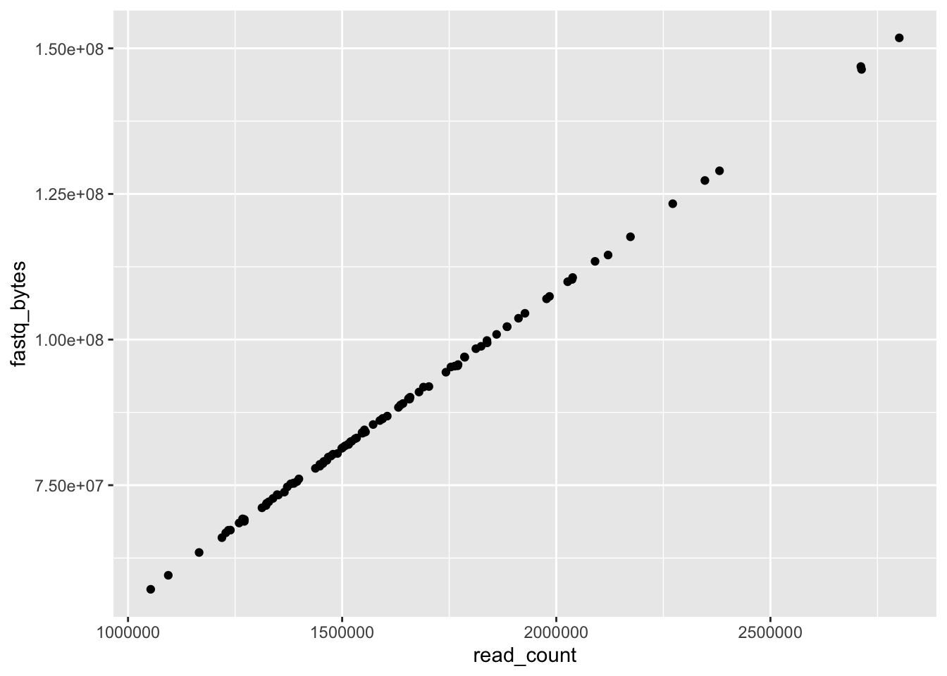
ggplot(data = yeast_metadata, mapping = aes(x = read_count, y = fastq_bytes)) +
  geom_point()
sets what type of plot we want to have (boxplot, lines, bars):
geom_point()for scatter plots, dot plots, etc.;geom_boxplot()for boxplots;geom_line()for trend lines, time series, etc.
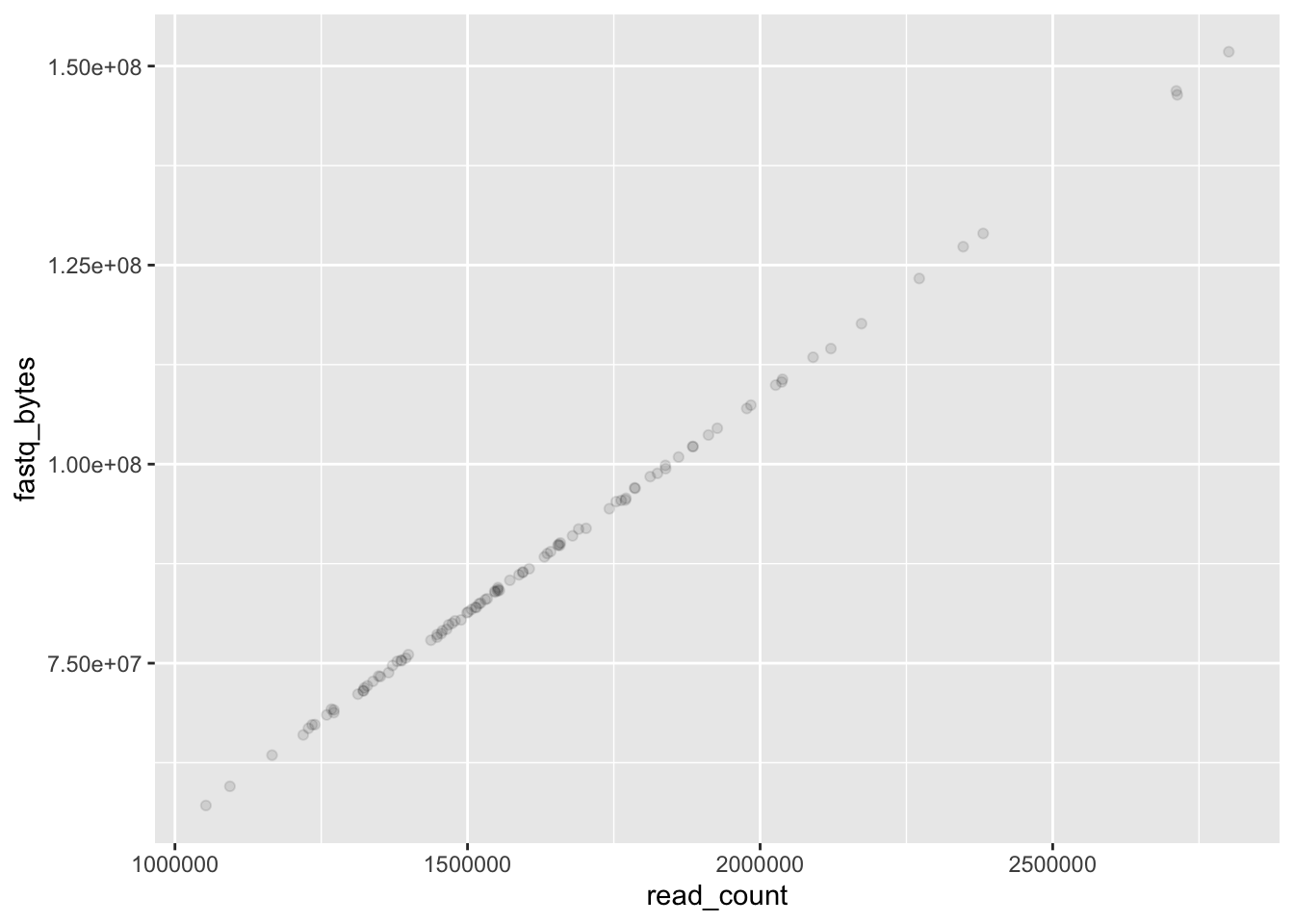
We can modify plots to extract more information. We can add transparency:
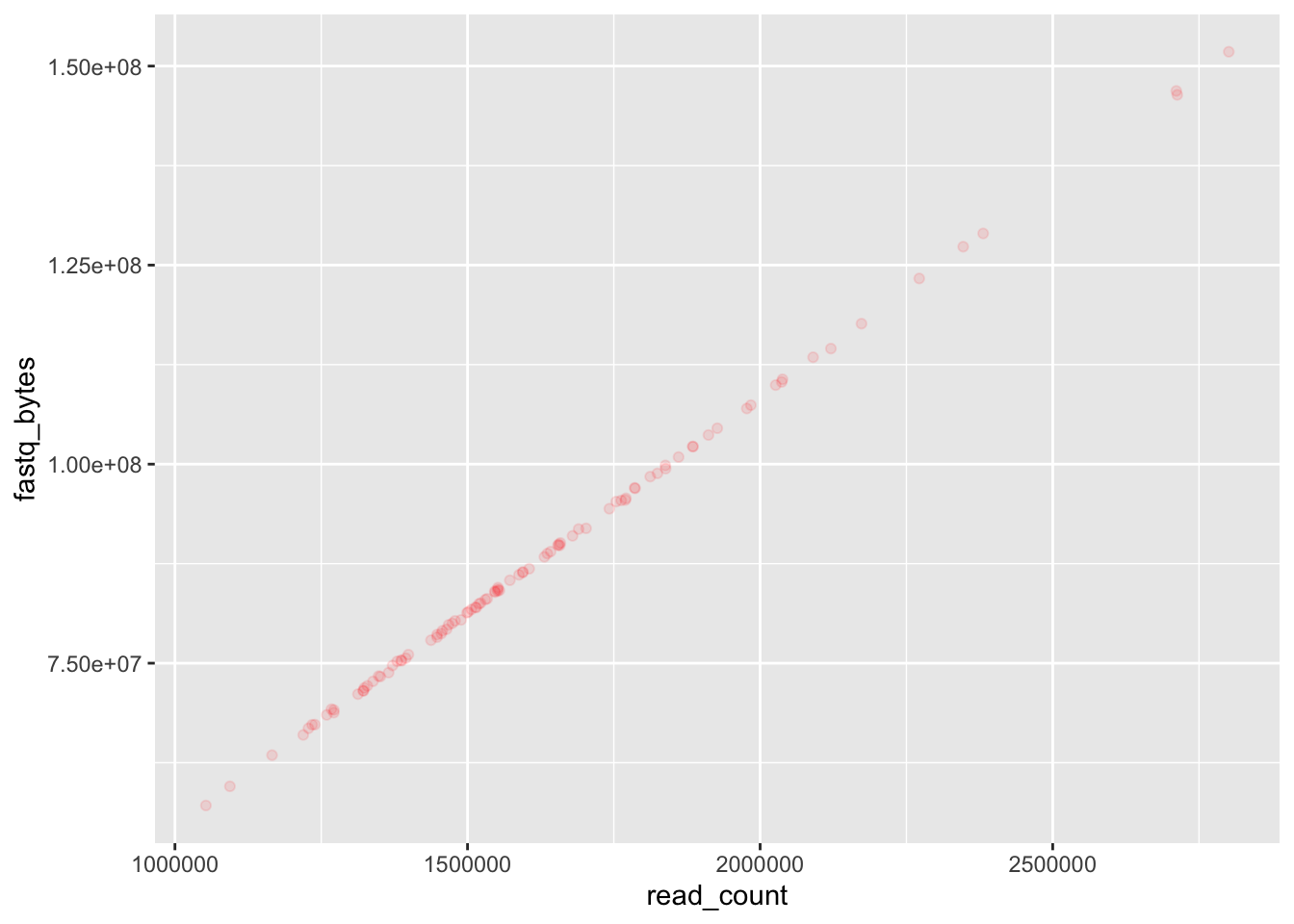
ggplot(data = yeast_metadata, mapping = aes(x = read_count, y = fastq_bytes)) +
  geom_point(alpha = 0.1)
or change the color of the points:
ggplot(data = yeast_metadata, mapping = aes(x = read_count, y = fastq_bytes)) +
  geom_point(alpha = 0.1, color = "red")
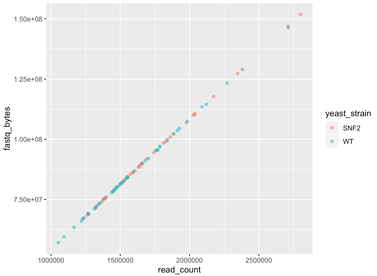
Or color each strain differently:
ggplot(data = yeast_metadata, mapping = aes(x = read_count, y = fastq_bytes)) +
  geom_point(alpha = 0.5, aes(color = yeast_strain))

We can also specify the color inside the mapping:
ggplot(data = yeast_metadata, mapping = aes(x = read_count, y = fastq_bytes, color = yeast_strain)) +
  geom_point(alpha = 0.5)
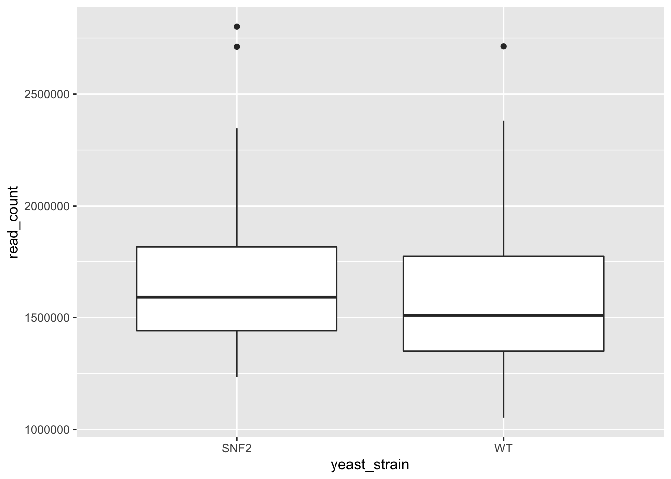
We can use boxplots to see the distribution of reads within strains:
ggplot(data = yeast_metadata, mapping = aes(x = yeast_strain, y = read_count)) +
  geom_boxplot()
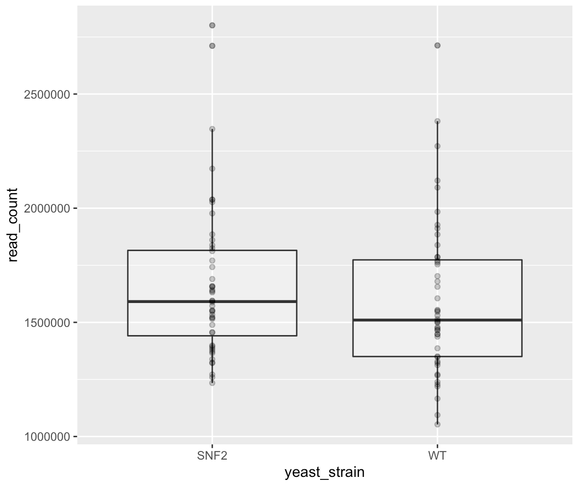
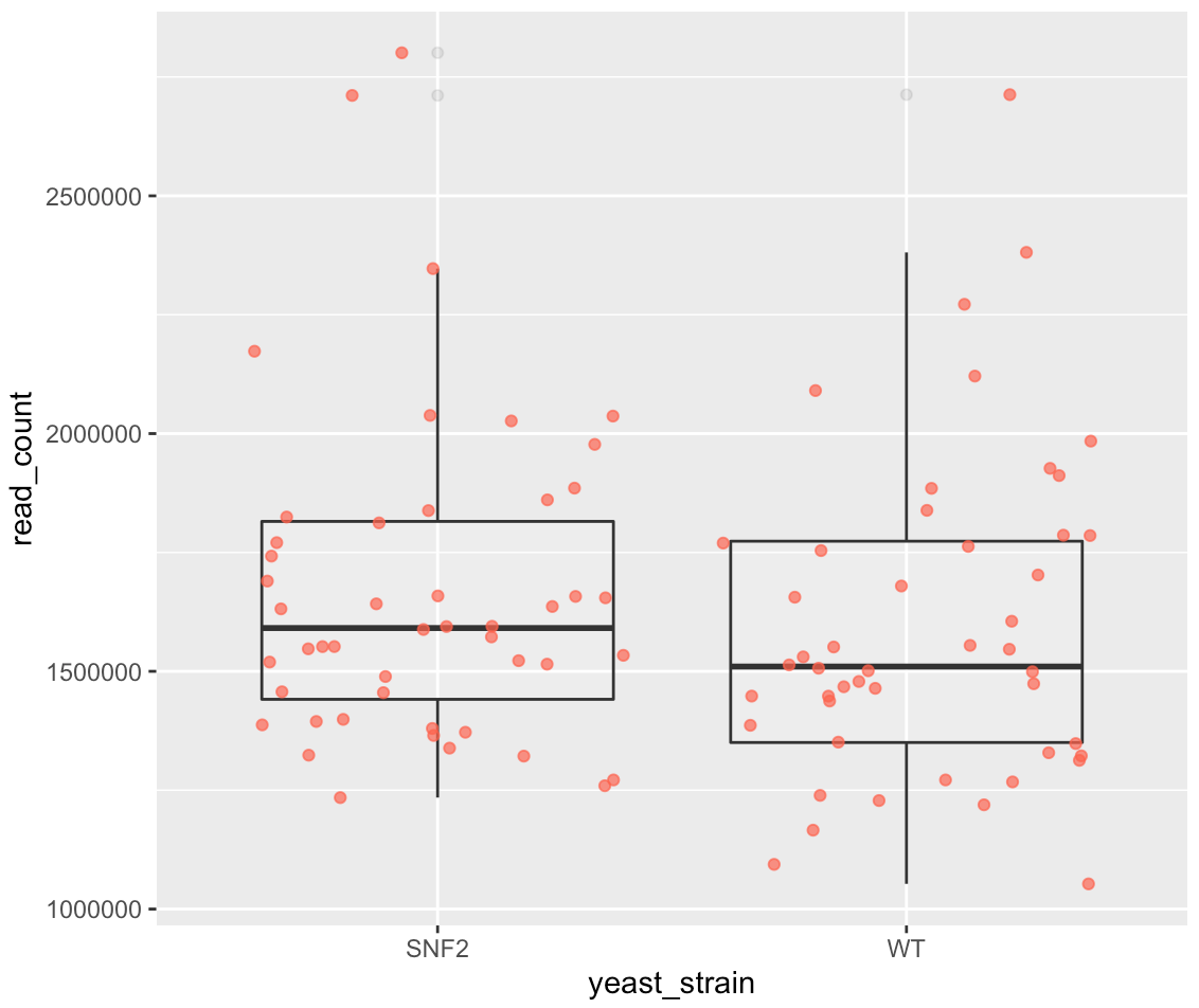
This is useful, but if we add dots to the boxplots we will have a better idea of the number of measurements and their distribution:
ggplot(data = yeast_metadata, mapping = aes(x = yeast_strain, y = read_count)) +
  geom_boxplot(alpha = 0.25) + geom_point(alpha = 0.25)
With categorical bins on the x-axis, we can also use geom_jitter() to spread out the points to be more clear:
ggplot(data = yeast_metadata, mapping = aes(x = yeast_strain, y = read_count)) +
  geom_boxplot(alpha = 0.1) + geom_jitter(alpha = 0.7, color = "tomato")
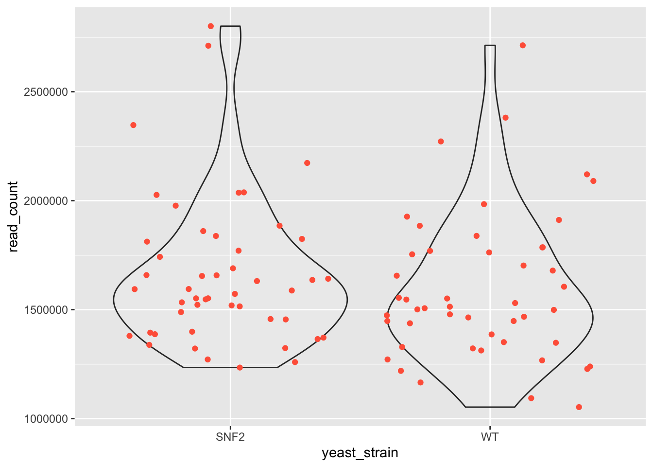
11.6.1. Exercise 10
Replace the boxplot with a violin plot.
Solution #10
ggplot(data = yeast_metadata, mapping = aes(x = yeast_strain, y = read_count)) +
  geom_violin(alpha = 0.1) +
  geom_jitter(alpha = 1, color = "tomato")
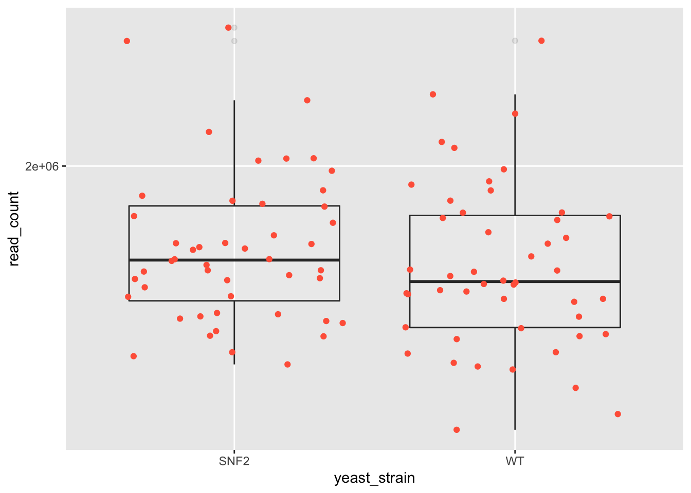
11.6.2. Exercise 11
Represent the read_count on log10 scale. Check out
scale_y_log10().
Solution #11
ggplot(data = yeast_metadata, mapping = aes(x = yeast_strain, y = read_count)) +
  scale_y_log10() +
  geom_boxplot(alpha = 0.1) +
  geom_jitter(alpha = 1, color = "tomato")
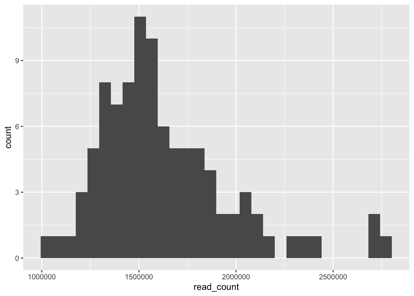
11.6.3. Exercise 12
Try to make a histogram plot for the read counts, coloring each yeast strain.
Solution #12
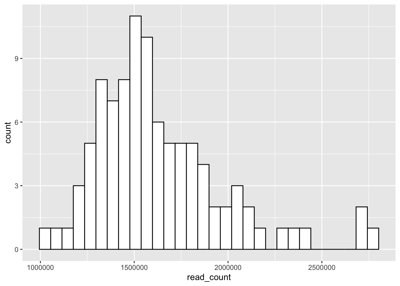
# Basic histogram
ggplot(data = yeast_metadata, aes(x=read_count)) +
  geom_histogram()
# Change colors
p<-ggplot(data = yeast_metadata, aes(x=read_count)) +
  geom_histogram(color="black", fill="white")
p
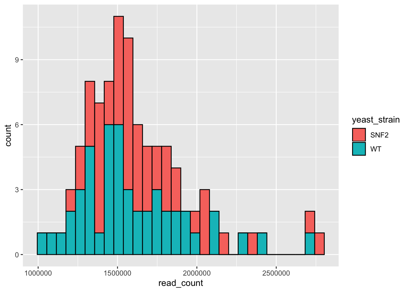
# Change colors based on yeast strain
ggplot(data = yeast_metadata, aes(x=read_count, fill = yeast_strain)) +
  geom_histogram(color="black")
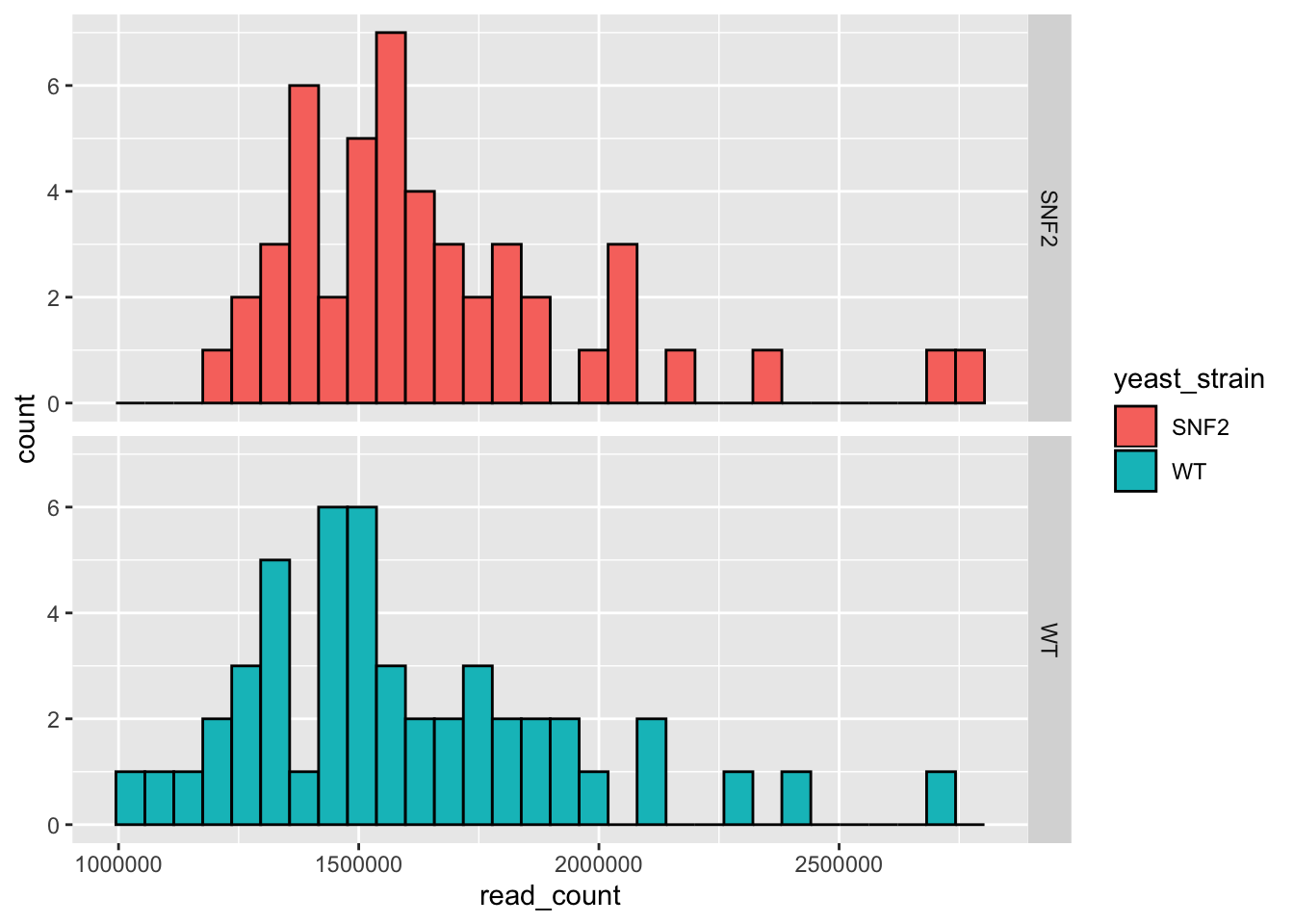
# Facet based on yeast strain
ggplot(data = yeast_metadata, aes(x=read_count, fill = yeast_strain)) +
  geom_histogram(color="black") +
  facet_grid(yeast_strain~.)
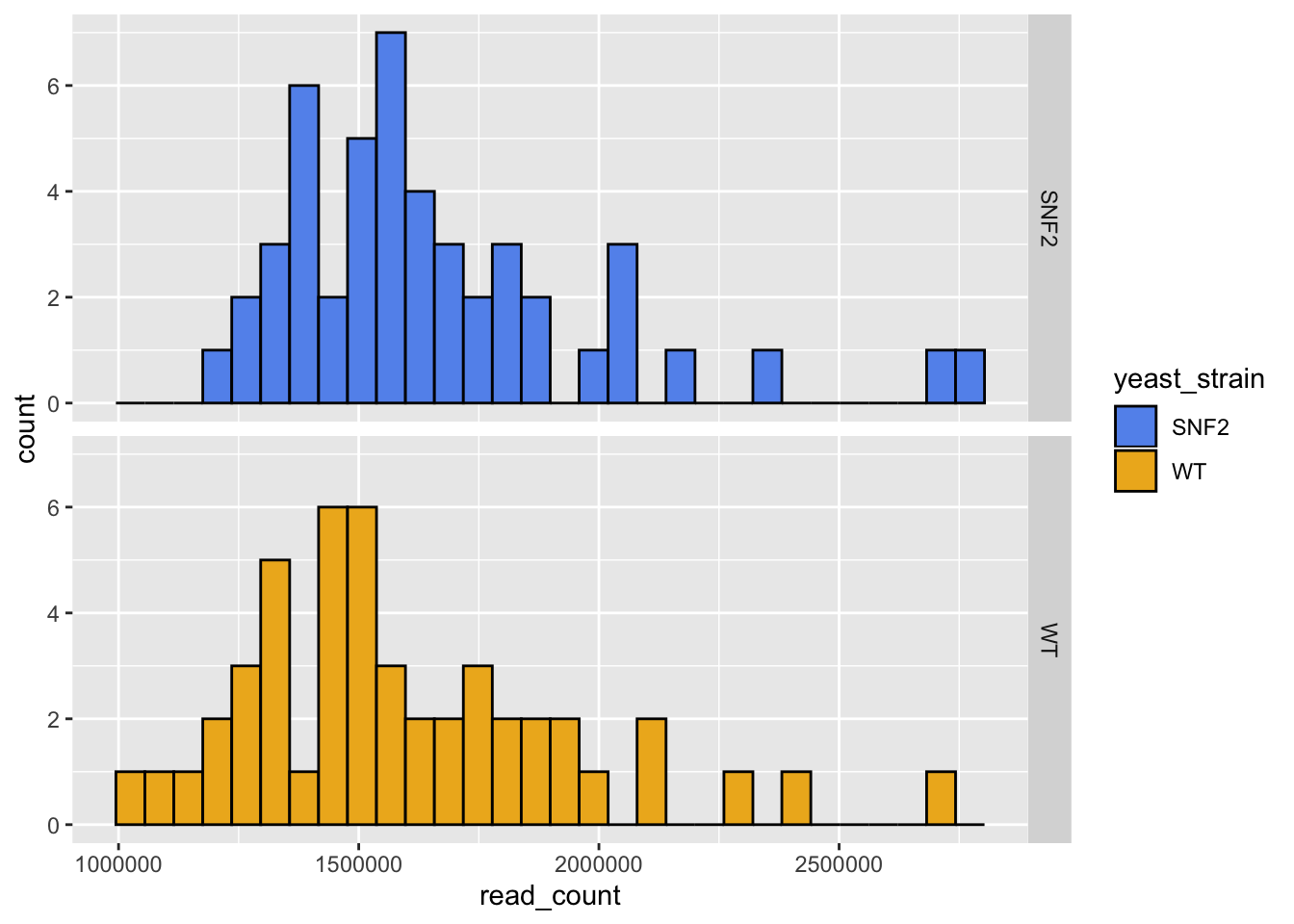
# Change to custom colors that are color blind friend
ggplot(data = yeast_metadata, aes(x=read_count, fill = yeast_strain)) +
  geom_histogram(color="black") +
  facet_grid(yeast_strain~.) +
  # Add blue and yellow colors that are more colorblind friendly for plotting
  scale_fill_manual(values = c("cornflowerblue", "goldenrod2"))
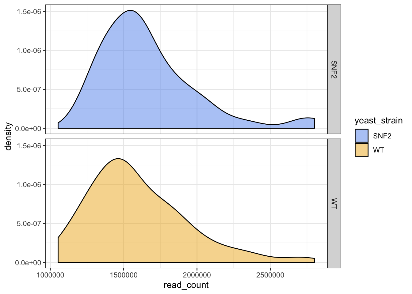
# Density based on yeast strain
ggplot(data = yeast_metadata, aes(x=read_count, fill = yeast_strain)) +
  facet_grid(yeast_strain~.) +
  geom_density(alpha = 0.5) +
  scale_fill_manual(values = c("cornflowerblue", "goldenrod2"))
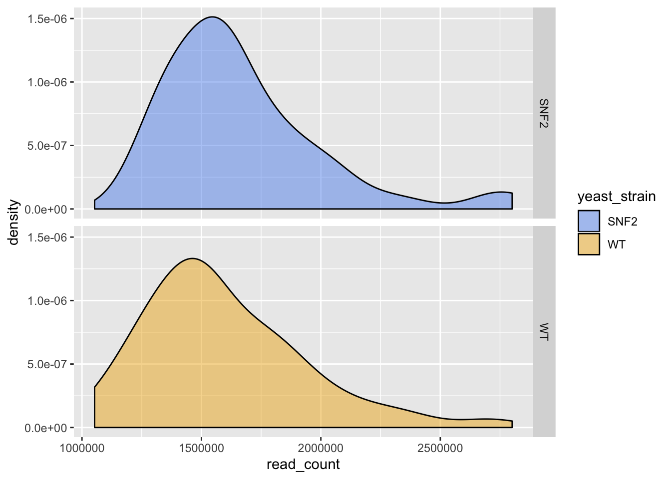
# A white background might be preferable for the yellow color
ggplot(data = yeast_metadata, aes(x=read_count, fill = yeast_strain)) +
  facet_grid(yeast_strain~.) +
  geom_density(alpha = 0.5) +
  scale_fill_manual(values = c("cornflowerblue", "goldenrod2")) +
  theme_bw()
11.6.4. Exercise 13
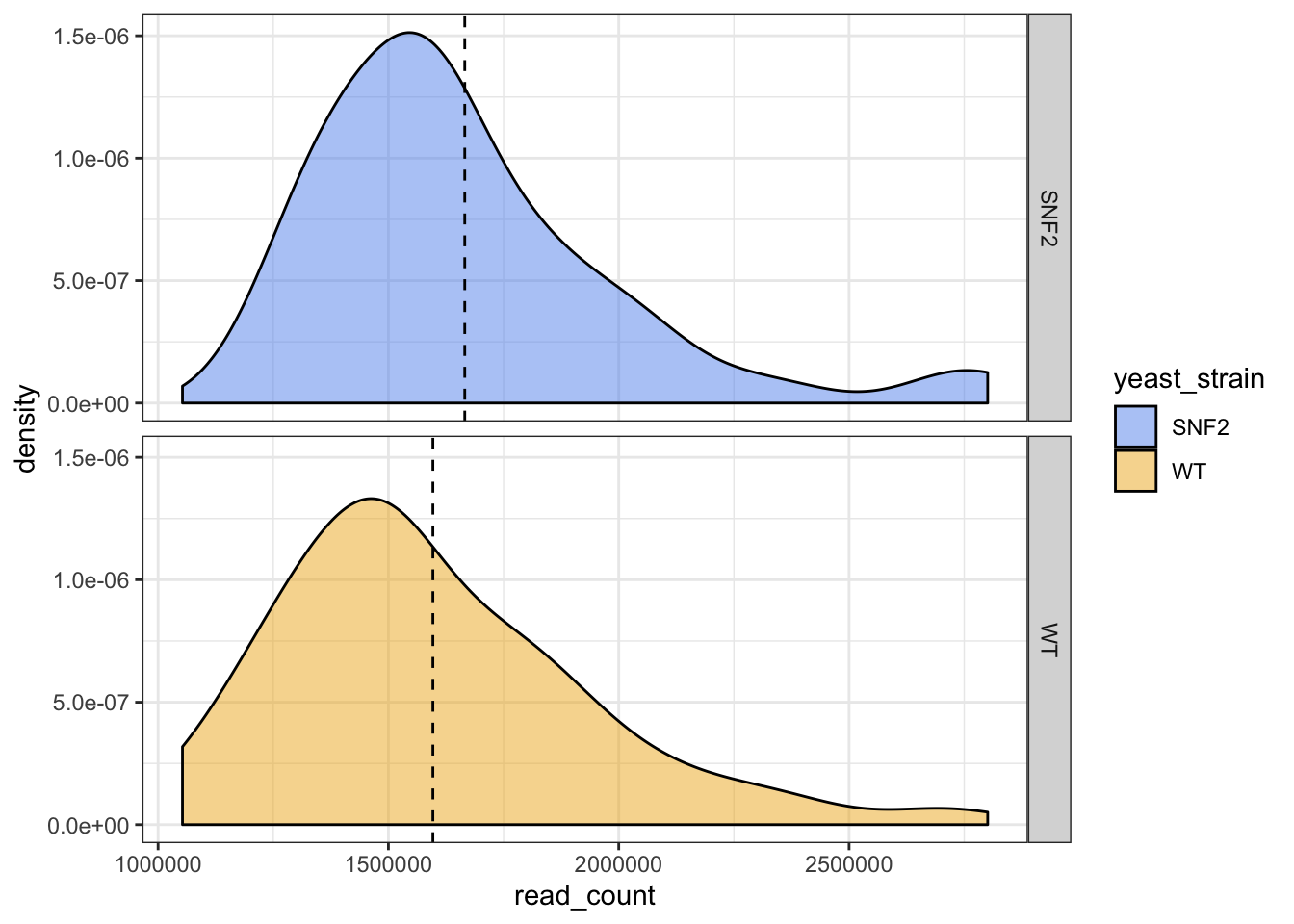
What if we want to add the mean read counts in a vertical line?
Solution #13
# To do so, we need to calculate the mean_read_count in a new data frame
mean_yeast_data <- yeast_metadata %>%
  group_by(yeast_strain) %>%
  summarise(mean_read_count = mean(read_count))
head(mean_yeast_data)
## # A tibble: 2 x 2
##   yeast_strain mean_read_count
##   <chr>                  <dbl>
## 1 SNF2                1665717.
## 2 WT                  1596525.
# Add the mean read_count with vline
ggplot(data = yeast_metadata, aes(x=read_count, fill = yeast_strain)) +
  geom_density(alpha = 0.5) +
  facet_grid(yeast_strain~.) +
  geom_vline(data = mean_yeast_data, mapping = aes(xintercept = mean_read_count),
             linetype="dashed", size=0.5) +
  theme_bw() +
  scale_fill_manual(values = c("cornflowerblue", "goldenrod2"))
11.7. Acknowledgements
This lesson was inspired by and adapted from the Data Carpentry Ecology R lessons
11.8. More material
=============
There are many amazing resources and cheat sheets to continue learning R, including: