12. Differential Expression and Visualization in R
Learning objectives:
Create a gene-level count matrix of Salmon quantification using tximport
Perform differential expression of a single factor experiment in DESeq2
Perform quality control and exploratory visualization of RNA-seq data in R
12.1. Getting started on Jetstream
You should still have your jetstream instance running, you can following the instructions here to log in to JetStream and find your instance. Then ssh into it following the instructions here.
You should have the salmon counts on your instance in the ~/quant/ folder. If
not, you can get this data by running:
cd ~
mkdir -p quant
cd quant
wget -O salmon_quant.tar.gz https://osf.io/5dbrh/download
tar -xvf salmon_quant.tar.gz
12.2. Importing gene-level counts into R using tximport
When we finished running salmon, we had a quant folder that contained
transcript-level read counts. So far in our RNA-seq pipeline, we have been
working from the command line in bash. For the rest of the RNA-seq tutorial,
we will be working in R. As we saw in the R introduction lesson, R is really
good and working with data in table format. When we produced counts for our
reads, we essentially transformed our data to this format. Most of the software
tools written to analyze RNA-seq data in this format are written in R.
We first need to read our data into R. To do that, we will use a package called
tximport.
This package takes transcript-level counts and summarizes them to the gene
level. It is compatible with many count input formats, including salmon.
First, launch RStudio from your instance. Run the following link to produce a url that navigates to RStudio when entered in your browser.
echo http://$(hostname -i):8787/
From R, start a new script.
Load the libraries tximport, DESeq2, and tidyverse so we have
access to the functions. We’ve pre-installed these packages for you, but we’ll
go over how to install them in the future.
library(tximport)
library(DESeq2)
library(tidyverse)
We need a couple files to import our counts.
First, we need a file that tells tximport where our files are. We’ve added
other information to this file about sample names and condition, which we will
also use later for differential expression. We can use the read_csv()
function to read this file into R as a dataframe directly from a url.
# read in the file from url
samples <- read_csv("https://osf.io/cxp2w/download")
# look at the first 6 lines
head(samples)
you should see output like this,
# A tibble: 6 x 3
  sample    quant_file                                condition
  <chr>     <chr>                                     <chr>
1 ERR458493 ~/quant/ERR458493.qc.fq.gz_quant/quant.sf wt
2 ERR458494 ~/quant/ERR458494.qc.fq.gz_quant/quant.sf wt
3 ERR458495 ~/quant/ERR458495.qc.fq.gz_quant/quant.sf wt
4 ERR458500 ~/quant/ERR458500.qc.fq.gz_quant/quant.sf snf2
5 ERR458501 ~/quant/ERR458501.qc.fq.gz_quant/quant.sf snf2
6 ERR458502 ~/quant/ERR458502.qc.fq.gz_quant/quant.sf snf2
Second, we need a file that specifies which transcripts are associated with which genes. In this case, we have associated transcript names with yeast ORF names.
# read in the file from url
tx2gene_map <- read_tsv("https://osf.io/a75zm/download")
# look at the first 6 lines
head(tx2gene_map)
the output should look something like this,
# A tibble: 6 x 2
  TXNAME                GENEID
  <chr>                 <chr>
1 lcl|BK006935.2_mrna_1 YAL068C
2 lcl|BK006935.2_mrna_2 YAL067W-A
3 lcl|BK006935.2_mrna_3 YAL067C
4 lcl|BK006935.2_mrna_4 YAL065C
5 lcl|BK006935.2_mrna_5 YAL064W-B
6 lcl|BK006935.2_mrna_6 YAL064C-A
We can now use tximport() to read in our count files
txi <- tximport(files = samples$quant_file, type = "salmon", tx2gene = tx2gene_map)
Let’s look at this new object:
summary(txi)
                    Length Class  Mode
abundance           36774  -none- numeric
counts              36774  -none- numeric
length              36774  -none- numeric
countsFromAbundance     1  -none- character
txi is a bit like a list, where it has multiple objects in it. Let’s take a
look at the counts:
head(txi$counts)
We have all of our counts in one place! One thing they’re missing is
informative column names. We can set these using our samples files, which will
also ensure that we assign the correct names to each column.
colnames(txi$counts) <- samples$sample
12.3. Why do we need to normalize and transform read counts
Given a uniform sampling of a diverse transcript pool, the number of sequenced reads mapped to a gene depends on:
its own expression level,
its length,
the sequencing depth,
the expression of all other genes within the sample.
In order to compare the gene expression between two conditions, we must therefore calculate the fraction of the reads assigned to each gene relative to the total number of reads and with respect to the entire RNA repertoire which may vary drastically from sample to sample. While the number of sequenced reads is known, the total RNA library and its complexity is unknown and variation between samples may be due to contamination as well as biological reasons. The purpose of normalization is to eliminate systematic effects that are not associated with the biological differences of interest.
Normalization aims at correcting systematic technical biases in the data, in order to make read counts comparable across samples. The normalization proposed by DESeq2 relies on the hypothesis that most features are not differentially expressed. It computes a scaling factor for each sample. Normalized read counts are obtained by dividing raw read counts by the scaling factor associated with the sample they belong to.
12.4. Differential Expression with DESeq2
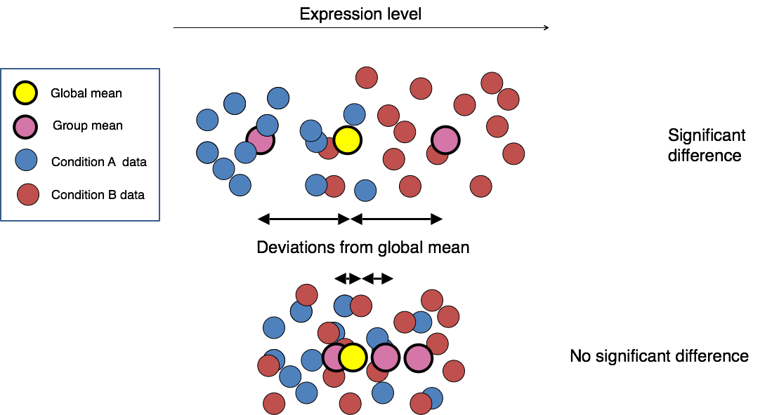
Image credit: Paul Pavlidis, UBC
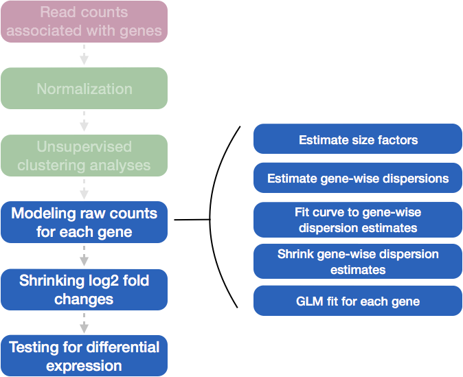
Differential expression analysis with DESeq2 involves multiple steps as displayed in the flowchart below. Briefly,
DESeq2 will model the raw counts, using normalization factors (size factors) to account for differences in library depth.
Then, it will estimate the gene-wise dispersions and shrink these estimates to generate more accurate estimates of dispersion to model the counts.
Finally, DESeq2 will fit the negative binomial model and perform hypothesis testing using the Wald test or Likelihood Ratio Test.
We’re now ready to use DESeq2, the package that will perform differential
expression.
We’ll start with a function called DESeqDataSetFromTximport which will
transform our txi object into something that other functions in DESeq2 can
work on. This is where we also give information about our samples contain
in the samples data.frame, and where we provide our experimental design. A design formula tells the statistical software the known sources of variation to control for, as well as, the factor of interest to test for during differential expression testing. Here our experimental design has one factor with two levels.
dds <- DESeqDataSetFromTximport(txi = txi,
                                colData = samples,
                                design = ~condition)
Note: DESeq stores virtually all information associated with your experiment in one specific R object, called DESeqDataSet. This is, in fact, a specialized object of the class “SummarizedExperiment”. This, in turn,is a container where rows (rowRanges()) represent features of interest (e.g. genes, transcripts, exons) and columns represent samples (colData()). The actual count data is stored in theassay()slot.
After running this command, you should see red output messages that look something like this:
using counts and average transcript lengths from tximport
Warning message:
In DESeqDataSet(se, design = design, ignoreRank) :
  some variables in design formula are characters, converting to factors
The first thing we notice is that both our counts and average transcript
length were used to construct the DESeq object. We also see a warning
message, where our condition was converted to a factor. Both of these
messages are ok to see!
Now that we have a DESeq2 object, we can can perform differential expression.
dds <- DESeq(dds)
Everything from normalization to linear modeling was carried out by the use of a single function! This function will print out a message for the various steps it performs:
estimating size factors
using 'avgTxLength' from assays(dds), correcting for library size
estimating dispersions
gene-wise dispersion estimates
mean-dispersion relationship
final dispersion estimates
fitting model and testing
And look at the results! The results() function lets you extract the base means across samples, log2-fold changes, standard errors, test statistics etc. for every gene.
res <- results(dds)
head(res)
log2 fold change (MLE): condition wt vs .
Wald test p-value: condition wt vs .
DataFrame with 6 rows and 6 columns
               baseMean     log2FoldChange             lfcSE               stat               pvalue                 padj
              <numeric>          <numeric>         <numeric>          <numeric>            <numeric>            <numeric>
ETS1-1 150.411380876596 -0.212379164913443 0.226307045512225 -0.938455824177912    0.348010209041573    0.670913203685731
ETS2-1                0                 NA                NA                 NA                   NA                   NA
HRA1   1.08884236321432   3.97189996253477  3.31146245569429   1.19943982928292    0.230356968252411                   NA
ICR1   28.8713313668145 -0.179654414034232 0.547534328578008 -0.328115343015677    0.742824453568867    0.907583917807416
IRT1   29.6053852845893  0.347498338858063 0.523744585645556   0.66348817416364    0.507017950920217    0.794457978516333
ITS1-1 23.8676180072013  -7.25640067170996  1.28178177600513  -5.66118258782368 1.50333365625958e-08 2.62112769016311e-07
The first thing that prints to the screen is information about the “contrasts” in the differential expression experiment. By default, DESeq2 selects the alphabetically first factor to the be “reference” factor. Here that doesn’t make that much of a difference. However, it does change how we interpret the log2foldchange values. We can read these results as, “Compared to SNF2 mutant, WT had a decrease of -0.2124 in log2fold change of gene expression.
Speaking of log2fold change, what do all of these columns mean?
| baseMean | giving means across all samples |
|---|---|
| log2FoldChange | log2 fold changes of gene expression from one condition to another. Reflects how different the expression of a gene in one condition is from the expression of the same gene in another condition. |
| lfcSE | standard errors (used to calculate p value) |
| stat | test statistics used to calculate p value) |
| pvalue | p-values for the log fold change |
| padj | adjusted p-values |
We see that the default differential expression output is sorted the same way as our input counts. Instead, it can be helpful to sort and filter by adjusted p value or log2 Fold Change:
res_sig <- subset(res, padj<.05)
res_lfc <- subset(res_sig, abs(log2FoldChange) > 1)
head(res_lfc)
12.5. Visualization of RNA-seq and Differential Expression Results
Looking at our results is great, but visualizing them is even better!
12.5.1. MA Plot
The MA plot provides a global view of the relationship between the expression change between conditions (log ratios, M), the average expression strength of the genes (average mean, A) and the ability of the algorithm to detect differential gene expression: genes that pass the significance threshold are colored in red
plotMA(res)
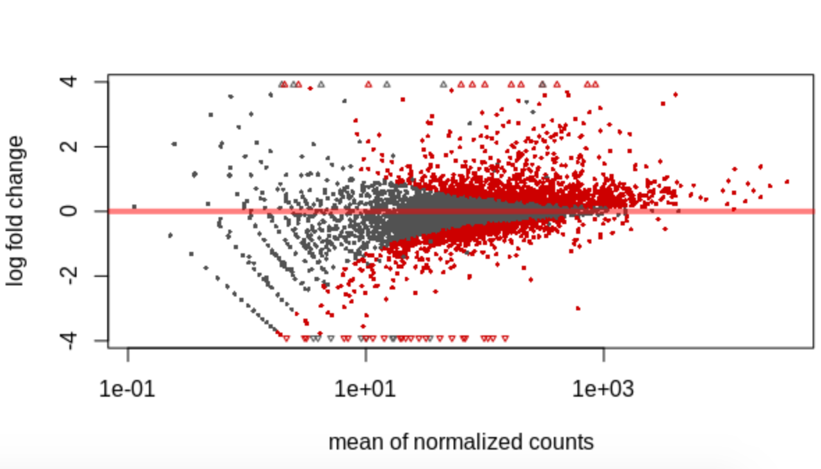
Question
Why are more genes grey on the left side of the axis than on the right side?
12.5.2. Plotting individual genes
Although it’s helpful to plot many (or all) genes at once, sometimes we want to see how counts change for a specific gene. We can use the following code to produce such a plot:
plotCounts(dds, gene=which.min(res$padj), intgroup="condition")
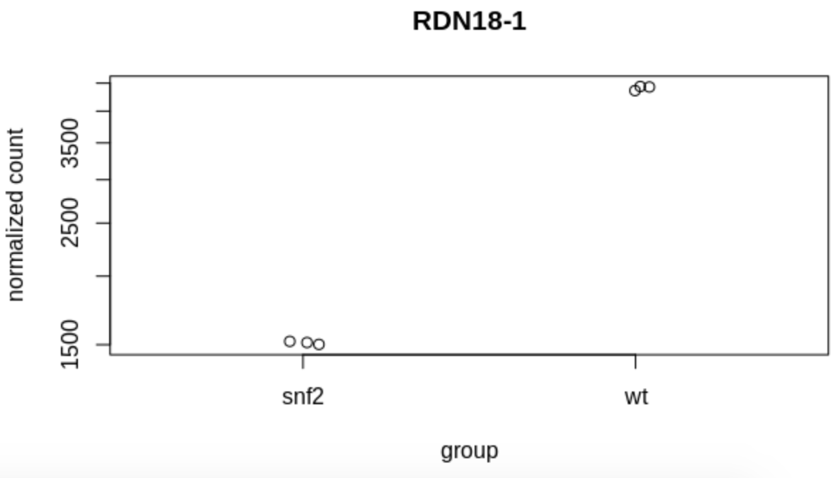
Question
What gene is plotted here (i.e., what criteria did we use to select a single
gene to plot)?
12.5.3. Normalization & Transformation
DESeq2 automatically normalizes our count data when it runs differential
expression. However, for certain plots, we need to normalize our raw count data.
One way to do that is to use the vst() function. It perform variance
stabilized transformation on the count data, while controlling for library
size of samples.
vsd <- vst(dds)
12.5.4. MDS Plot
An MDS (multi-dimensional scaling) plot gives us an idea of how our samples relate to each other. The closer two samples are on a plot, the more similar all of their counts are. To generate this plot in DESeq2, we need to calculate “sample distances” and then plot them.
# calculate sample distances
sample_dists <- assay(vsd) %>%
  t() %>%
  dist() %>%
  as.matrix()

head(sample_dists)
Next, let’s calculate the MDS values from the distance matrix.
mdsData <- data.frame(cmdscale(sample_dists))
mds <- cbind(mdsData, as.data.frame(colData(vsd))) # combine with sample data
head(mds)
And plot with ggplot2!
ggplot(mds, aes(X1, X2, shape = condition)) +
  geom_point(size = 3) +
  theme_minimal()
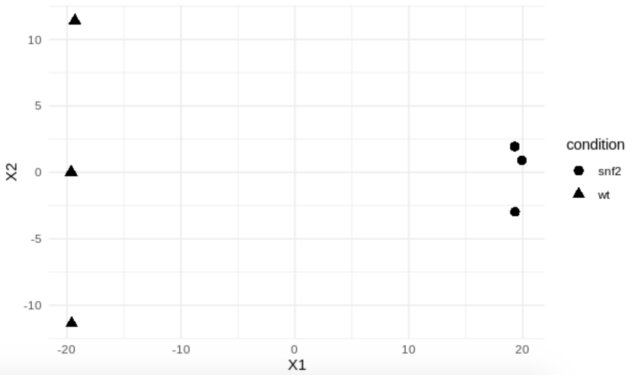
Question
How similar are the samples between conditions?
12.5.5. Heatmap
Heatmaps are a great way to look at gene counts. To do that, we can use a
function in the pheatmap package. Here we demonstrate how to install a
package from the CRAN repository and then load it into our environment.
install.packages("pheatmap")
library(pheatmap)
Next, we can select a subset of genes to plot. Although we could plot all ~6000 yeast genes, let’s choose the 20 genes with the largest positive log2fold change.
genes <- order(res_lfc$log2FoldChange, decreasing=TRUE)[1:20]
We can also make a data.frame that contains information about our samples that will appear in the heatmap. We will use our samples data.frame from before to do this.
annot_col <- samples %>%
  column_to_rownames('sample') %>%
  select(condition) %>%
  as.data.frame()

head(annot_col)
And now plot the heatmap!
pheatmap(assay(vsd)[genes, ], cluster_rows=TRUE, show_rownames=TRUE,
         cluster_cols=FALSE, annotation_col=annot_col)
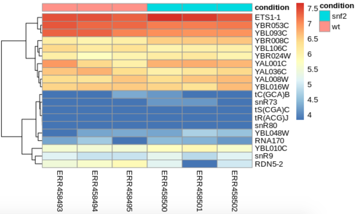
We see that our samples do cluster by condition, but that by looking at just the counts, the patterns aren’t very strong. How does this compare to our MDS plot?
Question
When are heatmaps useful?
What other types of heatmaps have you seen in the wild?
12.6. Further Notes
Here are some helpful notes or resources for anyone performing differential expression.
Introduction to differential gene expression analysis using RNA-seq (Written by Friederike Dündar, Luce Skrabanek, Paul Zumbo). Click here
Introduction to DGE - click here
12.6.1. Making a tx2gene file
Making a tx2gene file is often a little different for each organism. If your
organism has a transcriptome (or *rna_from_genomic.fna.gz file) on RefSeq,
you can often get the information from the *feature_table.txt.gz. You
might also be able to parse a gtf or gff file to produce the information you
need. This information is sometimes also found in the fasta headers of the
transcriptome file itself.